Hyperparameter Tuning

Introduction

In Chapter Introduction to Machine Learning, we mentioned that most machine learning models come with hyperparameters, which are settings that control the learning process. In fact, nearly all machine learning models include some form of hyperparameter. Even the Laplace estimator in a Naive Bayes model can be interpreted as a hyperparameter (see Chapter Naive Bayes).

In this chapter, we focus on one of the simplest yet most effective approaches for selecting these values in order to improve predictive performance. We discuss how to tune hyperparameters using scikit-learn, how this process is integrated into workflows, and how different hyperparameter settings can be compared in terms of predictive performance.

Hyperparameter Tuning with Regular Grid Search

The goal of hyperparameter tuning is to improve model performance on unseen data. In previous chapters, we introduced the main hyperparameter(s) for each machine learning method, but we typically assigned them fixed values without extensive justification. This was done primarily for simplicity. In practice, however, the optimal choice of hyperparameters depends on the specific dataset and prediction task, making hyperparameter tuning an important step in the machine learning workflow.

There are different approaches to hyperparameter tuning, meaning methods for finding appropriate values that lead to good predictive performance. In this chapter, we focus on the simplest and most widely used approach: the regular grid search. The idea is to pre-specify a set of candidate values for each hyperparameter and evaluate all possible combinations using resampling methods. Each combination is treated as a separate model, and its performance is estimated using, for example, cross-validation. The final choice is then based on the average performance across resamples.

For instance, in the case of a k-nearest neighbors (KNN) model, the main hyperparameters is the number of neighbors. A common rule of thumb is to set \(k\) to the square root of the number of observations. However, instead of relying on a single heuristic value, grid search allows us to systematically evaluate a range of values around this guideline. For example, if we have a dataset with 3000 observations, the square-root rule suggests a value of approximately 55. Using a regular grid approach, we would not only test this value, but also a set of nearby values, such as 10, 25, 50, 75, 100, and 150, to assess how sensitive model performance is to the choice of \(k\).

The main advantage of regular grid search is that it is easy to understand and implement while giving the user full control over the hyperparameter values being evaluated. Rather than relying on a heuristic or automated search strategy, the user explicitly specifies the candidate values for each hyperparameter and systematically evaluates all possible combinations. However, the main drawback is computational cost. As the number of hyperparameters increases, the total number of combinations grows multiplicatively. This can quickly become infeasible, especially for complex models or large datasets. For example, if we tune three hyperparameters and consider only five values for each, we already end up with 125 possible configurations, each of which would need to be evaluated using cross-validation. For this reason, grid search is often used with relatively small and carefully chosen parameter ranges rather than exhaustive exploration.

From a practical perspective, it is suggested to start with a relatively wide grid that covers a reasonable range of values for each hyperparameter. At this stage, the goal is not to find the exact optimum, but to understand how performance behaves across different regions of the parameter space. Once we identify values that lead to better performance, we can refine the grid by focusing on a narrower range with finer resolution.

As with resampling methods, it is important that hyperparameter tuning is performed entirely only within the training set. The test set should not be used during this process, as this would again introduce optimistic bias. Instead, we rely on validation set(s) or cross-validation performance to guide the selection of hyperparameters. Once the final configuration has been selected, the model is refit on the full training set using the chosen hyperparameters. This ensures that the model incorporates all available information before being evaluated on the test set, which remains the final and unbiased measure of performance.

Hyperparameter Tuning with Scikit-learn

With scikit-learn, hyperparameter tuning is implemented using pipelines combined with GridSearchCV. To see how this works, we import the customer_churn dataset. We then use train_test_split() to create training and test sets, and RepeatedStratifiedKFold to generate 5×3 repeated cross-validation folds:

import pandas as pd
import numpy as np
from sklearn.model_selection import train_test_split, RepeatedStratifiedKFold

# Importing customer_churn
customer_churn = pd.read_csv("https://raw.githubusercontent.com/Datakortex/Datasets/refs/heads/main/customer_churn.csv")

# Importing and pre-processing the dataset
customer_churn = customer_churn[["Recency", "Frequency", "Monetary_Value", "Churn"]].copy()
customer_churn["Churn_Label"] = np.where(customer_churn["Churn"] == 1, "Churn", "No Churn")

# Splitting customer_churn
training_set, test_set = train_test_split(
  customer_churn,
  test_size = 0.25,
  stratify = customer_churn["Churn_Label"],
  random_state=  999
)

# 5x3 (repeated) cross-validation folds
folds_rep_cv = RepeatedStratifiedKFold(n_splits = 5,
                                       n_repeats = 3, 
                                       random_state = 123)

We now define a KNN model as part of a pipeline, the same kind of object we introduced in the previous chapter to chain together preprocessing and model-fitting steps. Here, we combine a scaling step to standardize the predictors with the KNN model itself. Unlike a model fitted with a fixed value, here we leave the number of neighbors unspecified for now, since it will be optimized later through the grid search itself:

from sklearn.pipeline import Pipeline
from sklearn.preprocessing import StandardScaler
from sklearn.neighbors import KNeighborsClassifier

# Building a pipeline with preprocessing and the KNN model
knn_pipeline = Pipeline([
  ("scaler", StandardScaler()),
  ("knn", KNeighborsClassifier())
  ])

The output shows the pipeline with its two steps: scaling the predictors, followed by the KNN classifier. The number of neighbors is left at its default value for now—it doesn’t need an explicit placeholder, since GridSearchCV will override it with each candidate value during the search.

Since we are tuning this parameter, we need to define a set of candidate values. A simple way is to create a dictionary where the key matches the pipeline step name and hyperparameter name, joined by a double underscore (knn__n_neighbors). We use the range() function to generate a sequence of values, which is convenient because it avoids manually specifying each value. In our case, we generate values from 5 to 105 in steps of 10:

# Creating the grid of candidate hyperparameter values
knn_grid = {"knn__n_neighbors": list(range(5, 106, 10))}

We now apply cross-validation using GridSearchCV(). This evaluates multiple hyperparameter values instead of fitting a single fixed model. To do this, we pass our pipeline, the grid of candidate values, the cross-validation folds, and the metrics we want to evaluate. Since our class labels are strings ("Churn"/"No Churn") rather than 0/1, we build precision, recall, and F1 scorers that explicitly treat "Churn" as the positive class. GridSearchCV() does accept plain string shortcuts such as scoring = "f1", but those rely on scikit-learn’s default choice of positive class, which (as we just saw with roc_auc_score()) isn’t always the one we actually mean. The function make_scorer() lets us wrap each metric function together with pos_label = "Churn" baked in, so we don’t run into that issue here:

from sklearn.model_selection import GridSearchCV
from sklearn.metrics import make_scorer, precision_score, recall_score, f1_score

# Defining scorers with "Churn" as the positive class
scoring = {
  "precision": make_scorer(precision_score, pos_label = "Churn"),
  "recall": make_scorer(recall_score, pos_label = "Churn"),
  "f1": make_scorer(f1_score, pos_label = "Churn")
  }

The code below fits the grid search itself. For every candidate number of neighbors in knn_grid, GridSearchCV() fits knn_pipeline on each resample’s analysis set and scores it on the assessment set using all three scorers—essentially the same analysis/assessment logic behind cross_validate() earlier in the chapter, just repeated once per hyperparameter value instead of once overall. Since we’re tracking three metrics at once, refit = "f1" tells it which one should decide the winning hyperparameter value and be used to refit a final model on the full training set:

# Fitting resamples and tuning
knn_results = GridSearchCV(
  estimator = knn_pipeline,
  param_grid = knn_grid,
  scoring = scoring,
  refit = "f1",
  cv = folds_rep_cv
  )

knn_results.fit(
  training_set[["Recency", "Frequency", "Monetary_Value"]],
  training_set["Churn_Label"]
  )

Once fitting completes, knn_results.cv_results_ holds the full set of results—one row per candidate hyperparameter value, with columns like param_knn__n_neighbors (the value tested) and mean_test_precision, mean_test_recall, mean_test_f1 (the average score across all resamples, one column per scorer):

# Collecting cross-validation metrics
cv_results = pd.DataFrame(knn_results.cv_results_)

This comes back in “wide” format, with one column per metric sitting side by side. However, it’s more convenient to reshape it into “long” format: one row per (neighbor value, metric) combination, with a single mean column and a metric column identifying which score it is. We get there by slicing out each metric’s two relevant columns, renaming its score column to the shared name mean, tagging it with assign(metric = ...), and stacking all three slices with concat():

# Reshaping from wide to long format
metrics_summary = pd.concat([
  cv_results[["param_knn__n_neighbors", "mean_test_precision"]].rename(
    columns = {"mean_test_precision": "mean"}).assign(metric = "precision"),
    cv_results[["param_knn__n_neighbors", "mean_test_recall"]].rename(
      columns = {"mean_test_recall": "mean"}).assign(metric = "recall"),
      cv_results[["param_knn__n_neighbors", "mean_test_f1"]].rename(
        columns = {"mean_test_f1": "mean"}).assign(metric = "f1")
        ], 
  ignore_index = True).rename(
    columns = {"param_knn__n_neighbors": "neighbors"}
    )

# Printing knn_results
metrics_summary

	neighbors	mean	metric
0	5	0.77	precision
1	15	0.81	precision
2	25	0.82	precision
3	35	0.83	precision
4	45	0.83	precision
5	55	0.84	precision
6	65	0.84	precision
7	75	0.85	precision
8	85	0.85	precision
9	95	0.85	precision
10	105	0.86	precision
11	5	0.67	recall
12	15	0.67	recall
13	25	0.67	recall
14	35	0.67	recall
15	45	0.67	recall
16	55	0.66	recall
17	65	0.66	recall
18	75	0.65	recall
19	85	0.64	recall
20	95	0.64	recall
21	105	0.64	recall
22	5	0.72	f1
23	15	0.73	f1
24	25	0.74	f1
25	35	0.74	f1
26	45	0.74	f1
27	55	0.74	f1
28	65	0.74	f1
29	75	0.73	f1
30	85	0.73	f1
31	95	0.73	f1
32	105	0.73	f1

The resulting metrics_summary has three rows for every candidate number of neighbors—one each for precision, recall, and F1—which is exactly the shape we’ll need to color by metric in the next plot.

We can create a plot to visualize the results using Seaborn. This produces a summary plot of the resampling results across the tested hyperparameter values:

import seaborn as sns
import matplotlib.pyplot as plt

# Plotting modeling results
sns.lineplot(
  data = metrics_summary,
  x = "neighbors", 
  y = "mean",
  hue = "metric",
  marker = "o"
  )

# Changing axis labels
plt.xlabel("Number of Neighbors")
plt.ylabel("Score")

# Displaying plot
plt.show()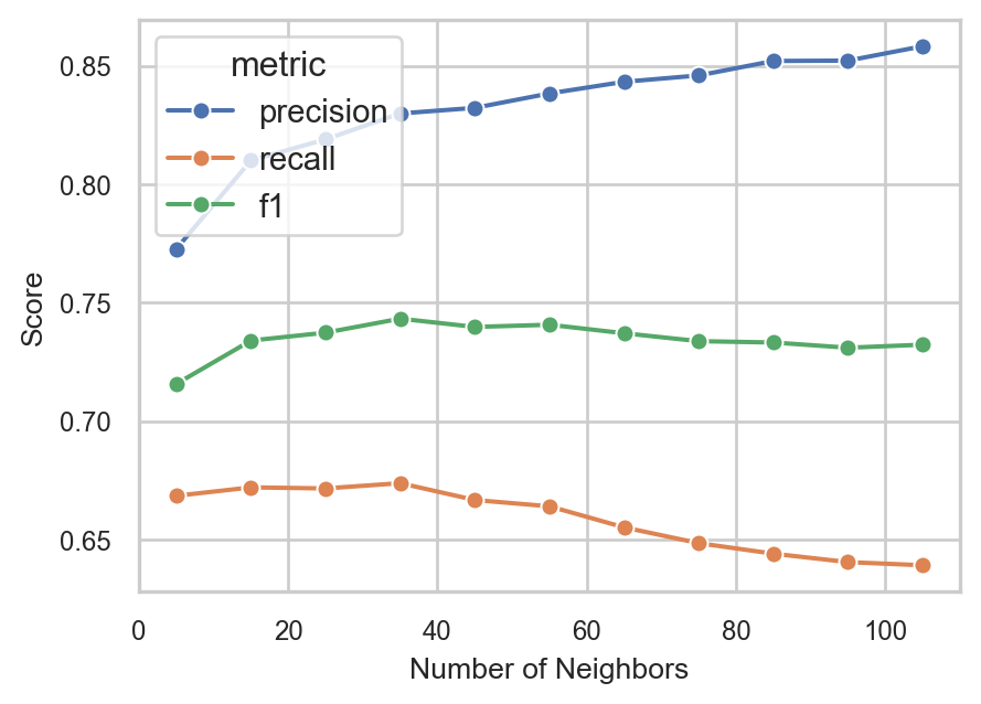

In this way, the results are shown across different values of neighbors, making it easy to compare model performance. Based on this visualization, 35 neighbors leads to the highest F1-score, with a precision above 80% and a recall between 65% and 70%. In practical terms, this means that around 80% of the predicted churners are actually correctly identified, while between 65% and 70% of all true churners are identified by the model.

Note that these are average values across the resamples, but based on our modeling setup, 35 neighbors appears to be a reasonable choice if this trade-off is acceptable from a business perspective. Interestingly, this choice also aligns with the common rule of thumb of using the square root of the number of observations as the number of neighbors in a KNN model.

We can extract the best-performing hyperparameters using the attribute best_params_. Since we set refit = "f1" above, this is already based on the F1-score:

# Selecting best hyperparameters
best_params = knn_results.best_params_

# Printing best_params
best_params

{'knn__n_neighbors': 35}

Unlike a two-step finalize-then-fit process, setting refit = "f1" in GridSearchCV() means the best-performing configuration is automatically refit on the full training set as soon as the grid search completes. This fitted model is available directly as knn_results.best_estimator_, fully specified and ready to evaluate—no separate finalization step is needed.

To evaluate the final model on the test set, we use knn_results.best_estimator_ to generate predictions and predicted probabilities. We then compute the same metrics as before, and additionally include roc_auc to measure the model’s ability to distinguish between the two classes across all classification thresholds.

Note that test_labels_numeric encodes the true labels as 0/1 with 1 = "Churn", matching what test_probabilities represents. However, roc_auc_score() has no pos_label argument to fall back on, so feeding it string labels directly would silently flip which class it treats as positive:

from sklearn.metrics import roc_auc_score

# Predicting on the test set using the best-performing model
test_predictions = knn_results.best_estimator_.predict(
  test_set[["Recency", "Frequency", "Monetary_Value"]]
  )
  
positive_class_index = list(knn_results.best_estimator_.classes_).index("Churn")

test_probabilities = knn_results.best_estimator_.predict_proba(
  test_set[["Recency", "Frequency", "Monetary_Value"]]
  )[:, positive_class_index]

# Encoding the true labels numerically, with 1 = "Churn" (matching test_probabilities)
test_labels_numeric = (test_set["Churn_Label"] == "Churn").astype(int)

# Collecting metrics
test_metrics = pd.DataFrame({
  "metric": ["roc_auc", "precision", "recall", "f1"],
  "estimate": [
    roc_auc_score(test_labels_numeric, test_probabilities),
    precision_score(test_set["Churn_Label"], test_predictions, pos_label = "Churn"),
    recall_score(test_set["Churn_Label"], test_predictions, pos_label = "Churn"),
    f1_score(test_set["Churn_Label"], test_predictions, pos_label = "Churn")
    ]})

# Printing results
test_metrics

	metric	estimate
0	roc_auc	0.90
1	precision	0.75
2	recall	0.62
3	f1	0.68

Disclaimer

It is strongly recommended to use the same set of metrics during both the training and testing phases to ensure consistency in model evaluation. In our example, we additionally include roc_auc at the testing stage to illustrate how ROC-based evaluation can be computed and visualized, even though it was not part of the tuning metrics.

The test metrics are slightly lower than the cross-validation results, which is expected. Some drop in performance is normal, since cross-validation provides an estimate based on resamples, while the test set represents completely unseen data. Lastly, we can use an ROC curve plot, a concept we discussed in Chapter Model Validation and Performance Evaluation. To do this, we use RocCurveDisplay.from_predictions() from scikit-learn, passing the true class labels and the predicted probabilities for the positive class ("Churn"), which are used to calculate and plot the curve in a single step:

from sklearn.metrics import RocCurveDisplay

# Plotting ROC curve
RocCurveDisplay.from_predictions(
  test_set["Churn_Label"],
  test_probabilities, 
  pos_label = "Churn"
  )

# Displaying plot
plt.show()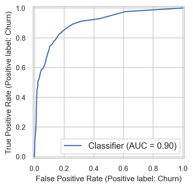

The ROC curve approaches the top-left corner of the plot, indicating a high true positive rate combined with a low false positive rate across many classification thresholds. This suggests that the model is able to distinguish well between the two classes, achieving both high sensitivity and strong specificity. This visual result is consistent with the roc_auc value of 0.9 obtained earlier, which summarizes the overall ability of the model to separate the positive and negative classes across all thresholds.

Recap

In this chapter, we focused on hyperparameter tuning using regular grid search. The idea is to systematically evaluate multiple combinations of hyperparameter values using resampling methods and select the configuration that performs best on average. We showed how this process is implemented in scikit-learn using pipelines and GridSearchCV(), and how the tuning process is integrated with cross-validation in a consistent framework.

We also highlighted the trade-off between simplicity and computational cost. While grid search is easy to understand and implement, it can quickly become expensive as the number of hyperparameters and candidate values increases. Finally, we demonstrated how the best-performing model is selected, automatically refit, and evaluated on a final test set to obtain an unbiased estimate of performance.