import pandas as pd

# Importing movies
movies = pd.read_csv("https://raw.githubusercontent.com/Datakortex/Datasets/refs/heads/main/Datacamp_public_datasets/movies.csv")Market Basket Analysis
Introduction
When browsing a product on an online marketplace (say Amazon), we’re often shown a list of recommended items. For example, after adding a laptop to the cart, we might be presented with suggestions for a mouse, a keyboard, or a laptop sleeve. A similar experience happens on platforms like Netflix or Disney Plus. Watching a movie often triggers recommendations for other titles with related themes or genres. If we watch the first The Lord of the Rings film, the sequel is likely to appear next.
It is not difficult to understand that these suggestions are anything but random. They’re powered by algorithms that learn from user behavior and preferences, in order to offer relevant recommendations (Schafer, Konstan, & Riedl, 2001; Adomavicius & Tuzhilin, 2005).
One of the most widely used techniques behind the generation of such recommendations is Market Basket Analysis (MBA). The core idea is simple: identify relationships between items that are frequently purchased together (Tan, Steinbach, & Kumar, 2019). In technical terms, we look for association rules—patterns like “if a customer buys product A, they’re also likely to buy product B”. These rules help businesses understand customer behavior and, therefore, improve cross-selling strategies.
Association Rules and Probability
In simple terms, an association rule shows that the purchase of one product increases the probability of purchasing another. For example, if many customers who buy product A also go on to buy product B, we can express this relationship as:
\[\{ \text{Product A} \} \Rightarrow \{ \text{Product B} \}\]
This reads as: “If product A is purchased, then product B is also likely to be purchased.” In other words, sale of product A implies sale of product B.
From a probability standpoint, association rules represent conditional probabilities. That means we’re interested in the probability that one event (e.g., buying product B) occurs, given that another event (e.g., buying product A) has already happened; we discussed how conditional probabilities apply to dependent events in Chapter Naive Bayes.
Here, each purchase is considered an event, and we want to know how the purchase of one product influences the probability of purchasing another. Mathematically, this is written as:
\[P(B \mid A)\]
We estimate this probability by checking how often product B is bought when product A has been bought. For instance, if 8 out of 10 customers who purchase product A subsequently purchase product B, we estimate the (conditional) probability of “B given A” as 80%.
Thinking Beyond Purchases
For the most part, we refer in this chapter to “purchases” in order to make the point clear to the reader. However, strictly speaking, we may be referring to “selections” or “basket additions”: when we add any item to our electronic basket, we are immediately presented with recommendations, even before our purchase has actually been concluded. Moreover, the reader is encouraged to think outside the analysis of a “market basket” to consider innovative applications of the same algorithm—that is one of the beauties (and utilities) of data science.
In many cases though, we need to visit more complex situations, such as how likely a customer is to buy product C given that they have already bought both product A and product B:
\[\{ \text{Product A, Product B} \} \Rightarrow \{ \text{Product C} \}\]
\[P(C \mid A, B)\]
As we start considering combinations of multiple products, the number of possibilities increases dramatically. For example, if a store offers 1,000 different products, there are 499,500 unique product pairs, and even more combinations when considering three or more items. Analyzing every possible combination would be computationally overwhelming and unnecessary, since many product combinations are irrelevant (for example, laptops and bicycles are rather unlikely to be selected for the same purchase transaction).
To deal with this complexity, we rely on smart algorithms, designed to filter out the noise and focus only on meaningful product combinations. One of the most popular algorithms for this task is the Apriori algorithm (Agrawal & Srikant, 1994), which is the approach we will use in this chapter.
Before we move on, it’s important to distinguish between market basket analysis and the Apriori algorithm. Market basket analysis is a data mining technique, its goal being to uncover association rules in transaction data. The Apriori algorithm, on the other hand, is a machine learning tool that helps us efficiently find such associations by calculating respective probabilities and filtering the results. In short, Apriori is one way to implement market basket analysis in practice.
Terminology and Assumptions
Before diving into the Apriori algorithm in Python, we need to clarify a few key terms and assumptions used in market basket analysis. Imagine observing customers at a supermarket checkout line. Each person holds a basket filled with items they’ve chosen. Some baskets might contain similar products, while others look completely different. In this setting, the contents of a single basket represent what we call an itemset, which is simply a group of items purchased simultaneously (Agrawal, Imieliński, & Swami, 1993).
In market basket analysis, we also use the term transaction. A transaction corresponds to a single shopping event—typically the set of items a single customer buys at one time. In our supermarket example, each basket is one transaction. Thus, the number of transactions equals the number of baskets we observe. This terminology is important because in practice we work with transactional data: a dataset where each row corresponds to one transaction (one basket), and the Apriori algorithm searching across all transactions to find frequent itemsets and association rules.
Respectively, let us focus on the main assumptions behind market basket analysis. While we could work around those assumptions depending on the question we want to ask, they help us start with and clarify the fundamentals and, at the same time, shape how we interpret and work with the data:
Quantity of a unit doesn’t matter: We don’t consider how many units of an item a customer buys. Whether someone purchases one can of milk or three, we treat it the same—we’re only interested in whether the item was bought (or not).
All items are treated equally: Every product is considered distinct, even if two items are very similar. For example, two different brands of toothpaste are treated just like two completely different products, such as bread and toothpaste; we don’t group items based on how similar they are.
Customers are open to recommendations: When we recommend product B because a customer has purchased product A, we assume the customer hasn’t already rejected product B. In other words, the association rule \({A} \Rightarrow {B}\) is only valuable if the customer is still open to buying B. This assumption is essential for the effectiveness of market basket analysis in real-world recommendation systems.
Understanding these assumptions helps us better interpret the results we get from the algorithm and gives us a solid foundation before we move on to implementation.
Applying the Apriori algorithm in Python
To apply the Apriori algorithm, we start by importing the movies dataset. The movies dataset is available on GitHub and consists of 5 columns (fields) and 17,575 rows (movies) that 100 users watched in an online platform. The 5 columns are as follows:
User_ID: ID number of the person that watched the movieMovie_ID: ID number of the movieTitle: Title of the movieYear: Release year of the movieGenres: Movie category
The key pieces of information we need for Market Basket Analysis are the column that identifies the customer and the column that lists the products purchased. These are the main variables used to build association rules. After importing the data, we pivot it so that we end up with one row per user (User_ID) and one column per movie (Title), with True indicating that the user watched that movie and False otherwise. We drop duplicate user-title pairs first, since a user who watched the same movie title more than once should still only count as one watch:
# Building the basket
movies_basket = (
  movies.drop_duplicates(subset = ["User_ID", "Title"])
  .assign(watched = True)
  .pivot(index = "User_ID", columns = "Title", values = "watched")
  .fillna(False)
  )

# Printing the first few rows and columns
movies_basket.iloc[0:2, 0:2]| Title | 'burbs, The | (500) Days of Summer |
|---|---|---|
| User_ID | ||
| 1323 | False | False |
| 1913 | False | False |
Because we are using the Title column instead of the Movie_ID column, movies that share the same title get collapsed into a single column, even though they may actually be different films. For example, King Kong has been released multiple times, in 1933, 1976, and 2005, with each version having a different Movie_ID. By using the Title column, we treat all movies with the same name as if they are the same, even though they are not. We do this for simplicity and better readability of the Apriori algorithm’s output, as it is easier to interpret the results (from a human perspective) when we see recognizable movie names rather than numeric IDs. However, this means that if a customer has watched both the 1933 and 2005 versions of King Kong, they are recorded as having watched it only once.
To get a better understanding of our data, we can look at its shape and at which movies were watched most often:
# Number of transactions (users) and items (movies)
movies_basket.shape
(100, 4382)# Most frequently watched movies
item_frequency = movies_basket.sum().sort_values(ascending = False)
# Printing the top 10 movies
item_frequency.head(10)Title
Matrix, The 60
American Beauty 57
Fight Club 54
Silence of the Lambs, The 50
Shawshank Redemption, The 48
Pulp Fiction 47
Lord of the Rings: The Fellowship of the Ring, The 45
Star Wars: Episode IV - A New Hope 44
Schindler's List 44
Sixth Sense, The 44
dtype: int64There are 100 transactions (users) and 4382 items (movies). The most frequent movies that were watched are The Matrix, American Beauty, Fight Club and The Silence of the Lambs. The movie The Matrix was watched by 60 users while American Beauty was watched by 57.
Visualizing Frequencies
We can visualize the most frequently watched movies (e.g. the top 10) directly from the original movies dataframe using countplot() from Seaborn. We sort the values first and plot them as a horizontal bar chart, since long movie titles are much easier to read this way than on a crowded x-axis:
import matplotlib.pyplot as plt
import seaborn as sns

# Getting the order of the top 10 movies
top10_order = movies["Title"].value_counts().head(10).index

# Plotting movie frequency
sns.countplot(
  data = movies[movies["Title"].isin(top10_order)],
  y = "Title",
  order = top10_order,
  color = "skyblue",
  edgecolor = "black"
  )

# Changing axis labels
plt.xlabel("Number of Users")
plt.ylabel("")

# Displaying plot
plt.show()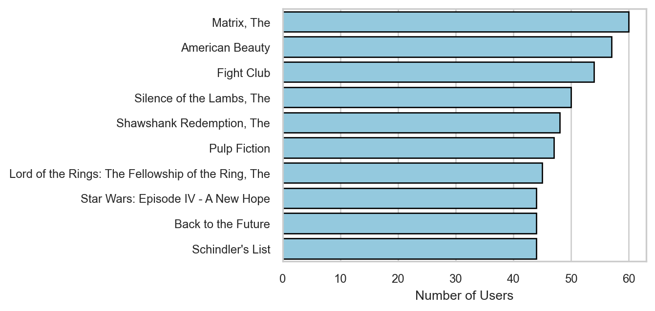
The most-watched movie is The Matrix, with 60 users, followed by American Beauty and Fight Club. Additionally, The Sixth Sense, Schindler’s List, and Back to the Future were all watched by the same number of users. Using the same approach, we can create similar frequency plots for other aspects of the dataset, such as the number of movies watched per user (basket_sizes, built above).
Support and Confidence
Two main characteristics guide market basket analysis: how often a product appears in the entire dataset, and how often one product appears after another one has already been selected. These are known as support and confidence, respectively.
Support is defined as the frequency an itemset occurs within all transactions (how much it is “supported”). Simply put, support tells us in how many baskets a product, or a combination of products, appears:
\[\text{Support(X)} = \frac{\text{Frequency(X)}}{N}\]
where \(X\) is an itemset and \(N\) is the number of transactions (or customers) the product appears. Essentially, support represents the probability that itemset \(X\) appears in a randomly selected basket:
\[\text{Support(X)} = P(X)\]
Confidence measures the strength of an association rule and is defined as the support of the combined itemset (\(X\), \(Y\)) divided by the support of \(X\) alone (how much confidence we have that product \(Y\) is also chosen given product \(X\) has been chosen). In other words, it is the conditional probability that product \(Y\) is purchased given that product \(X\) was purchased.
\[\text{Confidence}(X \to Y) = \frac{\text{Support}(X, Y)}{\text{Support}(X)} = \frac{\text{Frequency}(X, Y)}{\text{Frequency}(X)}\]
Mathematically, we have:
\[\text{Confidence}(X➔Y) = P(Y|X)\]
Note that confidence is directional: the confidence of \(X \to Y\) is different from \(Y \to X\), as the denominator differs.
Both support and confidence range between 0 and 1, as they represent probabilities. They form the basis for generating association rules, which are filtered using threshold values defined in advance. For example, we may choose to ignore rules involving products that are rarely purchased, by setting a minimum support. In this way, support and confidence also act as hyperparameters in market basket analysis.
To illustrate how this works, we will use the function apriori() from the mlxtend package. This function requires our basket (movies_basket) and a minimum support threshold. Suppose we want to find all itemsets with at least 30% support and containing at least three products (or movies in our example). Since apriori() only filters by support, we add the length condition ourselves afterwards:
from mlxtend.frequent_patterns import apriori, association_rules

# Applying the Apriori algorithm - Item frequency (support)
itemsets = apriori(movies_basket, min_support = 0.3, use_colnames = True)
itemsets["length"] = itemsets["itemsets"].apply(len)
To examine the results, we filter for itemsets with at least 3 movies and sort by support:
# Inspecting the results
itemsets[itemsets["length"] >= 3].sort_values("support", ascending = False)| support | itemsets | length | |
|---|---|---|---|
| 163 | 0.35 | (Lord of the Rings: The Two Towers, The, Lord ... | 3 |
| 160 | 0.34 | (Pulp Fiction, Fight Club, Silence of the Lamb... | 3 |
| 168 | 0.34 | (Star Wars: Episode V - The Empire Strikes Bac... | 3 |
| 165 | 0.33 | (Lord of the Rings: The Two Towers, The, Lord ... | 3 |
| 167 | 0.32 | (Pulp Fiction, Silence of the Lambs, The, Matr... | 3 |
| 154 | 0.31 | (Pulp Fiction, Silence of the Lambs, The, Amer... | 3 |
| 164 | 0.31 | (Lord of the Rings: The Fellowship of the Ring... | 3 |
| 169 | 0.31 | (Shawshank Redemption, The, Pulp Fiction, Sile... | 3 |
| 156 | 0.31 | (Back to the Future, Matrix, The, Star Wars: E... | 3 |
| 161 | 0.31 | (Forrest Gump, Silence of the Lambs, The, Matr... | 3 |
| 166 | 0.31 | (Lord of the Rings: The Two Towers, The, Matri... | 3 |
| 170 | 0.31 | (Lord of the Rings: The Two Towers, The, Lord ... | 4 |
| 152 | 0.30 | (Pulp Fiction, Fight Club, American Beauty) | 3 |
| 153 | 0.30 | (Pulp Fiction, American Beauty, Matrix, The) | 3 |
| 162 | 0.30 | (Jurassic Park, Silence of the Lambs, The, Mat... | 3 |
| 155 | 0.30 | (Matrix, The, Back to the Future, Raiders of t... | 3 |
| 159 | 0.30 | (Fight Club, Silence of the Lambs, The, Matrix... | 3 |
| 157 | 0.30 | (Fight Club, Lord of the Rings: The Fellowship... | 3 |
| 158 | 0.30 | (Pulp Fiction, Fight Club, Matrix, The) | 3 |
The itemsets column reflects the different itemsets found (e.g., the three Lord of the Rings movies), along with the columns support and length. The support column gives the probability of the itemset, and length simply counts how many movies are in it.
Since we have 100 users in our dataset, it’s easy to verify that support is calculated by dividing the frequency of an itemset by the total number of users. For example, the itemset with the highest support is the Lord of the Rings trilogy: 35 users (or 35% of all users in our dataset) watched all three movies. While it is intuitive that these three movies would frequently appear together, we haven’t created any (association) rules yet. Thus, we still don’t know, for instance, the probability that a user who watched the first movie also watched the second.
To generate association rules, we use association_rules() instead, applying it on the itemsets object we created earlier. Since association_rules() doesn’t expect the length column we added before, we drop it first. Let’s also set the min_threshold argument (which refers to the minimum required confidence) to 0.9, so as to emphasize only strong relationships:
# Applying the Apriori algorithm - Rules
rules = association_rules(
  itemsets.drop(columns = "length"),
  metric = "confidence",
  min_threshold = 0.9
  )

# Keeping rules with at least 3 movies across both sides
rules["total_items"] = rules["antecedents"].apply(len) + rules["consequents"].apply(len)
rules = rules[rules["total_items"] >= 3].drop(columns = "total_items")
The rules DataFrame contains all potential association rules. Each row has an antecedents column (the itemset \(X\), on the left-hand side) and a consequents column (the itemset \(Y\), on the right-hand side), so the statement “If customer selects itemset \(X\), then the customer will select itemset \(Y\)” maps directly onto these two columns, together with the support, confidence, and lift columns:
# Printing output
rules[["antecedents", "consequents", "support", "confidence", "lift"]]| antecedents | consequents | support | confidence | lift | |
|---|---|---|---|---|---|
| 8 | (Back to the Future, Raiders of the Lost Ark (... | (Matrix, The) | 0.30 | 0.94 | 1.56 |
| 9 | (Back to the Future, Star Wars: Episode IV - A... | (Matrix, The) | 0.31 | 0.94 | 1.57 |
| 10 | (Pulp Fiction, Fight Club) | (Silence of the Lambs, The) | 0.34 | 0.92 | 1.84 |
| 11 | (Fight Club, Silence of the Lambs, The) | (Pulp Fiction) | 0.34 | 0.92 | 1.96 |
| 12 | (Forrest Gump, Silence of the Lambs, The) | (Matrix, The) | 0.31 | 0.94 | 1.57 |
| 13 | (Jurassic Park, Silence of the Lambs, The) | (Matrix, The) | 0.30 | 0.91 | 1.52 |
| 14 | (Lord of the Rings: The Two Towers, The, Lord ... | (Lord of the Rings: The Return of the King, The) | 0.35 | 0.92 | 2.56 |
| 15 | (Lord of the Rings: The Two Towers, The, Lord ... | (Lord of the Rings: The Fellowship of the Ring... | 0.35 | 1.00 | 2.22 |
| 16 | (Lord of the Rings: The Fellowship of the Ring... | (Lord of the Rings: The Two Towers, The) | 0.35 | 1.00 | 2.63 |
| 17 | (Lord of the Rings: The Two Towers, The) | (Lord of the Rings: The Fellowship of the Ring... | 0.35 | 0.92 | 2.63 |
| 18 | (Lord of the Rings: The Return of the King, The) | (Lord of the Rings: The Two Towers, The, Lord ... | 0.35 | 0.97 | 2.56 |
| 19 | (Matrix, The, Lord of the Rings: The Return of... | (Lord of the Rings: The Fellowship of the Ring... | 0.31 | 1.00 | 2.22 |
| 20 | (Lord of the Rings: The Two Towers, The, Matri... | (Lord of the Rings: The Fellowship of the Ring... | 0.33 | 1.00 | 2.22 |
| 21 | (Lord of the Rings: The Two Towers, The, Matri... | (Lord of the Rings: The Return of the King, The) | 0.31 | 0.94 | 2.61 |
| 22 | (Matrix, The, Lord of the Rings: The Return of... | (Lord of the Rings: The Two Towers, The) | 0.31 | 1.00 | 2.63 |
| 23 | (Star Wars: Episode V - The Empire Strikes Bac... | (Star Wars: Episode IV - A New Hope) | 0.34 | 0.94 | 2.15 |
| 24 | (Star Wars: Episode V - The Empire Strikes Bac... | (Matrix, The) | 0.34 | 0.94 | 1.57 |
| 25 | (Lord of the Rings: The Two Towers, The, Lord ... | (Lord of the Rings: The Return of the King, The) | 0.31 | 0.94 | 2.61 |
| 26 | (Lord of the Rings: The Two Towers, The, Matri... | (Lord of the Rings: The Fellowship of the Ring... | 0.31 | 1.00 | 2.22 |
| 27 | (Lord of the Rings: The Fellowship of the Ring... | (Lord of the Rings: The Two Towers, The) | 0.31 | 1.00 | 2.63 |
| 28 | (Lord of the Rings: The Two Towers, The, Matri... | (Lord of the Rings: The Fellowship of the Ring... | 0.31 | 0.94 | 2.68 |
| 29 | (Matrix, The, Lord of the Rings: The Return of... | (Lord of the Rings: The Two Towers, The, Lord ... | 0.31 | 1.00 | 2.63 |
Each entry represents a rule in the form of “if X, then Y”, and since antecedents and consequents are sets of movie titles, movies whose titles contain commas (e.g. "Matrix, The") cause no parsing issues here.
Lift and Defining Association Rules
Setting the target argument to "rules", generates three additional columns: confidence, lift, and coverage. As previously discussed, confidence represents the conditional probability that the itemset on the right-hand side (consequent) is selected, given that the itemset on the left-hand side (antecedent) is selected. Coverage refers to the proportion of transactions in which both the antecedent and the consequent appear together. In simpler terms, it reflects how frequently both itemsets co-occur in the dataset and is effectively the support metric of the combined itemset. Lift, finally, is a particularly informative metric. Lift is defined as the support of the joint itemset (\(X\), \(Y\)) divided by the product of the individual supports of \(X\) and \(Y\). It quantifies how much more likely item \(Y\) is to be purchased given that item \(X\) is already purchased, relative to the overall probability of purchasing \(Y\).
The formula for lift is as follows:
\[\text{Lift}(X \to Y) = \text{Lift}(Y \to X) = \frac{\text{Support}(X, Y)}{\text{Support}(X) \times \text{Support(Y)}} = \frac{\text{Frequency}(X, Y)}{\text{Frequency}(X) \times \text{Frequency}(Y)}\]
Unlike confidence, lift is symmetric, meaning the direction of the rule does not matter:
\[\text{Lift}(X \to Y) = \text{Lift}(Y \to X)\]
Importantly, lift values above 1 indicate a positive association between the antecedent and the consequent: the presence of one increases the probability of the other occurring (Tan et al., 2019; Han, Kamber, & Pei, 2012). In our current output, all 18 association rules have a lift greater than 1, which suggests that each rule reflects a meaningful association. The higher the lift, the stronger the relationship between the items. However, since lift is derived from both support and confidence, the thresholds set for these two metrics directly affect which rules are generated and their corresponding lift values. Adjusting these thresholds will therefore influence the rules produced and their relative strength.
Rules on Specific Itemsets
Just as we can set a minimum number of items in an itemset, we can also restrict our analysis to rules involving specific items. In particular, we can specify that a certain item must appear on the left-hand side (antecedent) or right-hand side (consequent) of the association rule. For example, to generate rules where The Matrix appears on the right-hand side, we filter rules for rows where the consequent is exactly {Matrix, The}.
Both antecedents and consequents store their items as a frozenset—an immutable, unordered collection of items, used here because an itemset has no inherent order and shouldn’t be modified after it’s created. To check whether a row’s consequent matches The Matrix exactly, we therefore compare it against a frozenset containing that single title—in our case, The Matrix—rather than against a plain string or list:
# Rules for "Matrix, The"
matrix_rules = rules[rules["consequents"] == frozenset({"Matrix, The"})]

# Printing output
matrix_rules[["antecedents", "consequents", "support", "confidence", "lift"]]| antecedents | consequents | support | confidence | lift | |
|---|---|---|---|---|---|
| 8 | (Back to the Future, Raiders of the Lost Ark (... | (Matrix, The) | 0.30 | 0.94 | 1.56 |
| 9 | (Back to the Future, Star Wars: Episode IV - A... | (Matrix, The) | 0.31 | 0.94 | 1.57 |
| 12 | (Forrest Gump, Silence of the Lambs, The) | (Matrix, The) | 0.31 | 0.94 | 1.57 |
| 13 | (Jurassic Park, Silence of the Lambs, The) | (Matrix, The) | 0.30 | 0.91 | 1.52 |
| 24 | (Star Wars: Episode V - The Empire Strikes Bac... | (Matrix, The) | 0.34 | 0.94 | 1.57 |
As expected, only rules that have "Matrix, The" on the right-hand side are generated, since we explicitly filtered for this condition. The itemsets on the left-hand side can significantly “lift” the probability of "Matrix, The" being selected, with a lift value of approximately 1.5. Based on these insights, we might recommend the movie The Matrix to users who watched Star Wars: Episode IV – A New Hope and Star Wars: Episode V – The Empire Strikes Back.
Advantages and Limitations
Market Basket Analysis (MBA) is a simple and effective data mining method for understanding customer behavior and increasing interest in a company’s products. It can confirm intuitive patterns—such as customers who buy a laptop often also purchase a keyboard—validating assumptions and reinforcing business strategies. At the same time, some rules may initially seem surprising or even random. For instance, customers who buy a new laptop might also purchase a bicycle. While this association may appear spurious at first, it could reflect underlying behavior that is not immediately obvious, such as students relocating to a new city and adopting a new lifestyle. This highlights the importance of critically evaluating association rules, combining domain knowledge with statistical metrics like support, confidence, and lift.
Despite its usefulness and easy implementation, MBA has several limitations. Firstly, it identifies correlations, not cause-and-effect relationships, so associations must be interpreted with caution (Han, et al., 2012). MBA also typically ignores quantities, focusing only on whether items are purchased together, which can limit practical insights. Some rules, while statistically strong, may be irrelevant for business decisions or simply confirm what is already obvious, providing little new information, especially in small datasets (Lantz, 2023). Furthermore, most customers may not be responsive to recommendations, so even valid patterns may not translate into actual sales. Finally, in large datasets, MBA can generate a huge number of rules, making it challenging to identify actionable insights. For example, in a supermarket, the sheer number of potentially relevant product associations can make designing effective recommendations and optimizing shelf organization difficult (Agrawal et al., 1994).
To translate the findings of MBA into actionable insights, the focus should be on rules that are both statistically significant and practically relevant. In real-world applications, businesses can use Market Basket Analysis to optimize product placement in physical stores, tailor recommendations on e-commerce platforms, and design targeted promotions or bundled discounts. The ultimate goal is not merely to discover patterns, but to apply them in ways that enhance the customer experience and drive business success.
Recap
Market Basket Analysis (MBA) is a simple and effective data mining method for understanding customer purchasing behavior and improving product recommendations. It helps businesses identify patterns in transactions, which can be used for better product placement, cross-selling, and targeted promotions. To apply MBA in practice, we often use the Apriori algorithm, which efficiently finds association rules by calculating support, confidence, and lift, even in large datasets. While MBA can uncover both intuitive patterns and less obvious associations, it has limitations: it shows correlations, not causation, ignores purchase quantities, and can generate too many rules, some of which may be redundant or not useful. The key is to focus on rules that are both statistically meaningful and practically relevant, so that patterns can actually inform decisions and improve the customer experience.