Tree-Based Models
Introduction
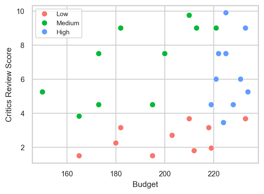
Imagine you work in a video game company and you are interested in finding out how you can predict whether the next video game will have “high”, “medium” or “low” success. Having data regarding the budget and the critics review score of other video games, you decide to visualize the data with the outcome of interest being the video game success:
The plot highlights that high budget and high critics review score usually lead to a video game that is of high success. With low critics review score, the game is usually of low success, even if the budget is high. With an average critics review score, the game can at least be of medium success.
Interestingly, with high critics review score and at least an average budget, a game is almost always a success. In other words, “if critics review score is more than x and the budget is more than y, then the game is of high success”. We can make similar statements for the other two levels of success. So, we can create a model that mimics the data using if-else statements. This is actually the intuition behind the Decision Tree method.
In this chapter, we explain the following machine learning methods: Decision Tree, Bagged Trees and Random Forest. Decision Tree is the foundation of tree-based models, while the other two methods are essentially advanced versions. Specifically, we discuss how this type of models are created, what their main hyperparameters are and how we can create such models in Python.
Decision Tree in Depth
Following the previous example, we want to fit a model that follows the if-else process we described. For simplicity, let’s try to use just one if-else statement. To represent an if-else statement in a plot, we draw only vertical or horizontal lines.
Although we could draw a vertical or horizontal line anywhere in this plot, such as where the average budget falls, we need to find a line that would provide meaningful insights. In our plot, one horizontal line that would make sense from a performance perspective is one that corresponds to a critics review score of 3.75:
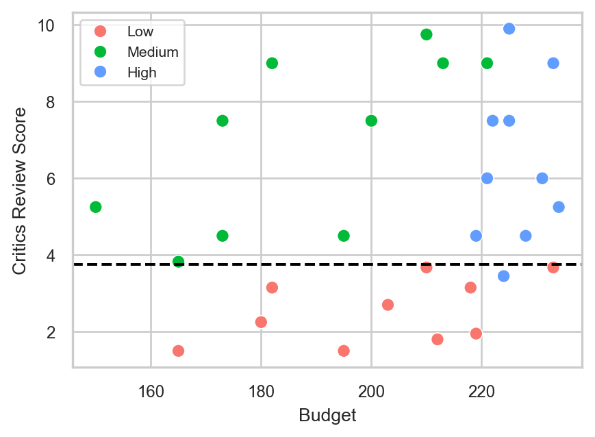
In this case, our statement would be the following: “if critics review score is higher than 3.75, a video game has a 91% probability of being of low success and 9% of being of high success, else it has 53% of being of medium success and 47% of being of high success”. These estimated probabilities derive from the proportion of the groups within each segment. For example, we have 11 games in total below the dashed line, out of which 10 are of low success and 1 is of high success. Therefore, 10 out of 11 video games within this segment are of low success, leading to a probability (proportion) of approximately 90%; all the estimated probabilities were estimated in the same way.
Our goal is to draw these lines that maximize the homogeneity (similarity) of the observations within each segment. Before this decision line on the plot, the probability that a game is of low success was 33%, but with this line, our estimated probability increases to 91%. Similarly, the probability of a game being of medium success before this line was 33%, but after creating this line, the probability rises to 53%. The main point is that using the two predictors, we manage to create an if-else scenario to increase the probability of detecting the success group of a video game.
We can continue this process and draw another line to split the data in more pieces. The second best line would be the following:
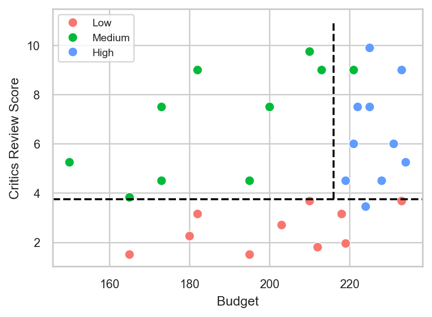
Having this more complex decision tree model, our estimated probabilities increase even more. We managed to create even more homogeneous segments. With this more complex model, we have the following scenarios:
Critics review score \(\le\) 3.75: 90% of low success and 10% of high success
Critics review score \(>\) 3.75 & Budget \(\le\) 216: 100% of medium success
Critics review score \(>\) 3.75 & Budget \(>\) 216: 90% of high success and 10% of medium success
Notice how the second line does not touch the x-axis; this line touches our first line because that was the optimal point in this example. However, the lines should create independent segments, meaning the lines should be perpendicular to either lines we created or the initial dimensional lines (e.g. x-axis).
The observations (data points on the plot) are not completely separated, and this should not be our goal either. Remember from the bias-variance trade off that our goal is to have a model with low bias and low variance. Adding more lines would lead to a decision tree that would learn this dataset too well (zero bias) but probably would not perform well on new data (very high variance). If we continue creating more segments, we will end up creating a separate segment for each observation.
With these two decision lines, our estimated probabilities for each segment have improved, meaning that the groups of games within each segment are more homogeneous. This illustrates the core idea behind a decision tree in supervised machine learning: recursively splitting the data to increase the purity of the outcome within each segment.
Because a decision tree is essentially a series of if-else statements, we cannot easily express the structure of the model mathematically (Kuhn et al., 2013). To express a decision tree, we can actually visualize its if-else statements in a tree-branch structure. For example, the decision tree that we described can be visualized like this:
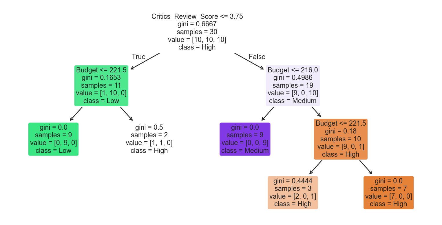
This plot describes the if-else statements we described earlier. If critics review score is below 3.75, then the game is of low success since the corresponding box has:
- 10 games are of low success
- 0 games are of medium success
- 1 game is of high success
Regarding the terminology, the “boxes” in the plot are called nodes, which reflect information about the proportion of each class within each created area of the decision tree. In Figure 19.4, the percentages reflect the proportion of the observations that belong to this node. For example, the node that has been created with critics review score lower than 3.75, includes 11 (or 36.67%) out of the 30 observations. When a node is the last one, it is also called leaf node and so all three nodes that we have can be called leaf nodes. The lines that form the boxes in the scatter plot are called splits or internal nodes. Lastly, the connections between nodes are called branches, which show the path of a decision from one node to the next or to a leaf.
It is apparent now why this type of modeling is called decision tree: the output visually resembles a tree structure, where decisions are made at each internal node, leading to different branches of possible outcomes.
At this stage, it makes sense to ask two questions: How do we know which lines are the optimal ones, and what do we mean by “optimal”? Although we could try to find these lines manually in this simple graph, it would be nearly impossible to do so when there are many more independent variables and observations. To solve this, we need an algorithm that uses a metric to determine the best splits automatically. The most well-known algorithm for this task is CART (Classification And Regression Trees). This algorithm is one of the earliest and most widely used algorithms for decision trees, and it is the one we focus on in this chapter, although other similar algorithms exist, such as C5.0, which we do not cover here.
Splitting Criteria in Classification Problems
For making the splits, the CART algorithm needs a specific criterion. Put differently, we have to determine a mathematical way of determining which split is considered better than the rest of potential splits. There are different splitting criteria depending on the algorithm and the machine learning task.
For classification tasks, the CART algorithm commonly uses Gini impurity as one of its criteria for splitting nodes in decision trees, particularly for classification tasks. Gini impurity is a measure of how often a randomly chosen observation from the set would be incorrectly labeled if it was randomly labeled according to the distribution of labels in the subset. To understand what this means it is important to firstly check the mathematical formula. The Gini (\(G\)) impurity for a node \(t\) with \(K\) classes can be calculated using the following formula:
\[G(t) = 1 - \sum_{i=1}^{K}{p(i|t)^2}\]
where \(p(i|t)\) represents the probability of randomly selecting an observation of class \(i\) from \(K\) classes from node \(t\). Let’s see a very simple example to understand how this formula works. Suppose that we have a dataset of 5 observations: 3 are of class A and 2 are of class B:
# Example data frame
gini_example = pd.DataFrame({
  "x": ["A", "A", "A", "B", "B"]
  })

# Printing results
gini_example| x | |
|---|---|
| 0 | A |
| 1 | A |
| 2 | A |
| 3 | B |
| 4 | B |
With no other information, the probability that we randomly draw an observation of class A is 60% since 3 out of 5 observations are of class A. Consequently, the probability that we randomly draw an observation of class B is 40%. Therefore, the Gini impurity value is the following:
\[G(t) = 1 - (P_A^2 + P_B^2) = 1 - (0.6^2 + 0.4^2) = 1 - (0.36 + 0.16) = 1 - 0.52 = 0.48\]
If all the observations had one class only, then the probability of drawing an observation of that class would be 100% and, as a result, the Gini impurity would be 0. Therefore, Gini impurity measures how mixed the classes in a node are, and can take values between 0 and 1. Similarly to a Naive Bayes model, a decision tree model incorporates the additional variables to try to find the optimal solution. So, the goal of the algorithm is to minimize the Gini impurity, making as homogeneous nodes as possible.
Regarding its process, the CART algorithm minimizes Gini impurity by iteratively evaluating potential splits in the data and selecting the split that maximally reduces impurity. More specifically, the CART algorithm uses the following process:
1. Initial Node: At the beginning, CART starts with the entire dataset at the root node (the first node) of the decision tree.
2. Variable Selection: For each candidate variable, CART considers all possible split points. For categorical variables, each unique category is considered as a potential split point. For continuous variables, CART typically sorts the variable values and considers splitting at each distinct value or at midpoints between adjacent values.
3. Impurity Calculation: CART evaluates the impurity of the dataset before the split (parent node) and the impurity of the resulting subsets after the split (child nodes). It uses the Gini impurity formula to calculate impurity for each node.
4. Impurity Reduction: CART calculates the impurity reduction—how similar the observations are within a node after a split—achieved by each potential split. This is computed by subtracting the weighted sum of impurities of the child nodes from the impurity of the parent node. We should not forget that the Gini impurity at each node is different; it is possible that in a split, the Gini impurity can be 0 at one node but almost 1 in the other node.
5. Selecting the Best Split: CART chooses the split that maximizes the impurity reduction. In other words, it selects the split that results in the greatest decrease in impurity.
6. Recursive Process: After selecting the best split, CART recursively applies the same procedure to each resulting child node until a stopping criterion is reached. This may include a maximum tree depth, a minimum number of observations per node, or other rules designed to prevent overfitting. In tree-based models, these stopping rules are treated as hyperparameters.
By repeatedly selecting splits that lead to the greatest reduction in impurity, CART constructs a decision tree that effectively separates the data into homogeneous subsets with respect to the target variable, resulting in a powerful predictive model for classification tasks.
Splitting Criteria in Regression Problems
Similar to classification tasks, CART tries to create nodes in which the data points are as similar as possible based on a continuous variable. In regression problems, the predicted value for a node is the average of the target values of all observations in that node. For example, if a leaf node contains 5 observations with values {1, 2, 3, 4, 5}, the predicted value for that node would be 3.
For regression tasks, CART uses a different splitting criterion than in classification. Instead of Gini impurity, it typically uses Mean Squared Error (MSE) to evaluate the quality of a split. The MSE measures the average squared difference between the actual target values and the predicted values for a set of observations. Mathematically, for a node containing \(n\) observations with actual values \(y_{i}\) and predicted value \(\hat{y}\) (the node mean), the MSE is:
\[\text{MSE} = \frac{1}{n} \sum^n_{i = 1} (y_{i} - \hat{y}) ^ 2\]
When building a regression tree, CART seeks to minimize the MSE at each node by selecting the split that produces the largest reduction in MSE. Essentially, the algorithm evaluates all possible splits for each predictor and chooses the one that creates the most homogeneous child nodes in terms of the target variable.
The overall process of tree construction remains the same as in classification: the tree is grown recursively, until a stopping criterion is met (e.g., minimum number of observations in a node, maximum depth, or minimal decrease in MSE). After the tree is built, the predicted value for each leaf node is simply the average of the target variable for the observations that fall into that node.
This approach ensures that each split reduces the overall variance of the target variable within the resulting nodes, which is the regression analogue of creating “pure” nodes in classification.
Treating Binary Targets as Numeric in Regression Trees
The same idea applies when our dependent variable takes values of 0 and 1. Although this is technically a classification problem, we can treat the target as numeric to calculate probabilities in the nodes. In this case, the predicted value for a node is simply the average of the 0s and 1s in that node, which corresponds to the estimated probability of the outcome being 1. For example, if a leaf node contains 5 observations with values {1, 1, 1, 0, 0}, the predicted value would be 0.6 (or 60%) for any new observation that falls into that node. However, using this approach, the splits are determined based on MSE rather than Gini impurity, meaning that the resulting tree may differ slightly from a standard classification tree, since the numeric approach minimizes variance rather than class impurity.
Assumptions and Considerations
Tree-based models are relatively flexible and make fewer strict assumptions compared to other machine learning methods. However, there are some important considerations to keep in mind when applying them:
Variable Independence: Tree-based models do not require the features (variables) to be independent of each other. In fact, they can naturally capture interactions between variables through their hierarchical structure. However, when predictors are highly correlated, the model may become unstable in the sense that small changes in the data can lead to different variables being selected for splits, even if they carry similar information. This can affect the interpretability of the model as well as the predictive performance.
Variable Importance: Tree-based models implicitly assume that the predictors contain useful information for the prediction task. Irrelevant or noisy features can lead to overfitting or poor model performance, as the algorithm may select them for splits that do not generalize well to new data.
Hierarchical Partitions: The models assume that the underlying data structure can be approximated through a series of hierarchical splits. Each node represents a decision based on a feature, leading to a partitioning of the feature space into smaller and more homogeneous regions.
Homogeneity within Nodes: Tree-based models aim to create nodes where the observations are as similar as possible with respect to the target variable. This is why criteria such as Gini impurity (for classification) and MSE (for regression) are used: they guide the algorithm toward splits that increase the homogeneity of the resulting nodes, improving predictive accuracy.
Overall, tree-based models offer a flexible and interpretable approach to predictive modeling, but these considerations are important to keep in mind. Highly correlated predictors can reduce interpretability, while irrelevant features can lead to unstable or unnecessary splits. In practice, careful feature selection and model tuning can help mitigate these issues and improve the performance of the model.
Decision Tree in Python
To apply the decision tree method in Python, we use the DecisionTreeClassifier() class from the sklearn.tree module, which is based on the CART algorithm. We also use functions from matplotlib to visualize the structure of the resulting tree. Along with these libraries, we import the customer_churn dataset from GitHub
Since we want to predict whether a customer churns, we convert the original binary Churn variable into a categorical variable (Churn_Label). If the original value is 1, we assign the label "Churn", and if it is 0, we assign "No Churn". Next, we separate the predictors from the target variable and split the data into training and test sets using the train_test_split() function from sklearn.model_selection:
import pandas as pd
import numpy as np
from sklearn.model_selection import train_test_split

# Importing customer_churn
customer_churn = pd.read_csv("https://raw.githubusercontent.com/Datakortex/Datasets/refs/heads/main/customer_churn.csv")

# Creating column Churn_Label
customer_churn["Churn_Label"] = np.where(customer_churn["Churn"] == 1, "Churn", "No Churn")

X = customer_churn[["Recency", "Frequency", "Monetary_Value"]]
y = customer_churn["Churn_Label"]

# Split data into training and test sets
X_train, X_test, y_train, y_test = train_test_split(
  X, y, test_size = 0.25, random_state = 35
  )
Because decision trees make splits based on thresholds along a single variable at a time, the scale of the features does not affect the model. Therefore, tree-based models require no scaling of the data, unlike distance-based models such as KNN.
Except for the predictors and the training data, the DecisionTreeClassifier() class allows us to specify hyperparameters that control the complexity of the tree, similar to how n_neighbors controls the complexity of a KNN model. Tree-based models usually have many hyperparameters, depending on the algorithm and the implementation. Two of the most common hyperparameters are min_samples_split, which specifies the minimum number of observations required for a node to be split, and max_depth, which limits the maximum number of levels the tree can grow.
We can now use the DecisionTreeClassifier() class to create a decision tree on the customer churn dataset, using the numeric variables Recency, Frequency, and Monetary_Value as predictors. We set the hyperparameters min_samples_split and max_depth to 500 and 20, respectively:
from sklearn.tree import DecisionTreeClassifier

# Creating the decision tree model
dt_model = DecisionTreeClassifier(
  min_samples_split = 1000,
  max_depth = 20,
  random_state = 35
  )

# Training the decision tree
dt_model.fit(X_train, y_train)
To visualize the decision tree, we use the plot_tree() function from the sklearn.tree module. We provide the trained model object and specify additional arguments to improve the readability of the visualization, such as displaying feature names, class names, and rounding numerical values:
from sklearn.tree import plot_tree
import matplotlib.pyplot as plt

# Visualizing the decision tree
plt.figure(figsize = (10, 5))

plot_tree(
  dt_model,
  feature_names = X.columns,
  class_names = dt_model.classes_,
  filled = True,
  rounded = True,
  precision = 4
  )

plt.show()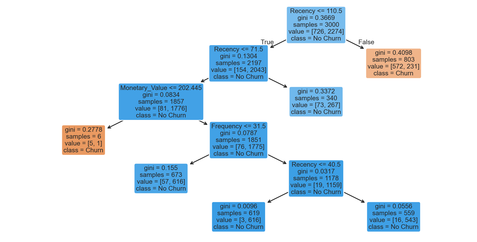
Focusing on the first split, we see that the majority of the observations fall in the node where Recency is lower than approximately 110. In that node, the predicted class is "No Churn" since 2043 out of 2197 observations belong to this class. The predicted class of the leaf node where Recency is higher than 110.5 is "Churn", as 572 out of 803 observations have this class. The first split already indicates that Recency is the most important predictor. Additionally, the outcome is easy to interpret: customers who have not made a purchase in the last approximately 4 months are much more likely to churn than those whose most recent purchase was within the last 4 months.
Let’s see now how we can use this model to make predictions on the test set. As we did in the previous chapters, we will use overall accuracy to measure the performance of our model on the test set. To generate predictions, we use the predict() method of the trained model, and to compute accuracy we use the accuracy_score() function from sklearn.metrics:
from sklearn.metrics import accuracy_score

# Making predictions on the test set
y_pred = dt_model.predict(X_test)

# Calculating accuracy
accuracy = accuracy_score(y_test, y_pred)

# Printing accuracy
accuracy0.869The model achieves an accuracy of approximately 87% on the test set, which is relatively good for such a simple model and substantially higher than the baseline NIF (always predicting the majority class), which is around 73%.
Bagged Trees
Our previous example highlighted that even a simple decision tree can provide good performance and interpretable results. However, one major challenge with decision trees is their tendency to overfit the data. This happens because a single tree can be highly sensitive to small variations in the training data. To address this, researchers developed a method to make decision trees more stable and prevent overfitting. The idea is simple: instead of relying on a single unstable model, we build many trees and then average their predictions. Intuitively, this approach is related to the Law of Large Numbers: as we increase the number of independent trees, the aggregated prediction converges to a more stable and accurate estimate (Breiman, 1996).
Of course, repeatedly fitting a decision tree on the exact same dataset would yield nearly identical trees. To introduce variability, we use bootstrapping, a resampling method where observations are randomly drawn with replacement from the original dataset. For example, if we have a dataset of 100 rows, bootstrapping allows us to create a new dataset of 100 rows where some observations may appear multiple times and some may not appear at all. Each bootstrap sample is similar, but not identical, to the original dataset.
We then fit a decision tree on each bootstrap sample. Since the datasets differ, each tree is slightly different. When making predictions, each tree casts a “vote” for the class of a given observation, and the final predicted class is determined by majority vote.
This process—resampling the data, fitting a decision tree on each sample, and aggregating predictions—is what we call bagged trees. Essentially, bagging is the combination of many decision trees trained on different datasets, each voting for the final outcome. We still use the CART algorithm and Gini impurity (for classification) or MSE (for regression) as splitting criteria, so all concepts discussed for single decision trees still apply.
In Python, we implement bagged trees using the BaggingClassifier() class from the sklearn.ensemble module. This method fits multiple decision trees on bootstrap samples of the training data and aggregates their predictions. The number of trees is controlled by the n_estimators parameter, while the complexity of each tree is defined through a decision tree specified as the base estimator, using hyperparameters such as min_samples_split and max_depth. In our case study, we fit 100 trees and set a random seed to ensure reproducibility:
from sklearn.ensemble import BaggingClassifier

# Setting seed for reproducibility
np.random.seed(1234)

# Defining base model (decision tree)
base_tree = DecisionTreeClassifier(
  min_samples_split = 1000,
  max_depth = 20,
  random_state = 1234
  )

# Bagged trees model
bt_model = BaggingClassifier(
  estimator = base_tree,
  n_estimators = 100,
  random_state = 1234
  )

# Training the model
bt_model.fit(X_train, y_train)
Unlike a single decision tree, bagged trees are not easily visualized because the model is an ensemble of many trees rather than one simple structure. The main advantage is increased predictive performance and stability, as the aggregation of multiple trees reduces variance and mitigates overfitting. The trade-off, however, is interpretability: unlike a single tree, we cannot easily see which splits or rules are driving the predictions.
We can make predictions and evaluate the model using the same functions as before:
# Making predictions on the test set
y_pred = bt_model.predict(X_test)

# Calculating accuracy
accuracy = accuracy_score(y_test, y_pred)

# Printing accuracy
accuracy0.87The accuracy does not seem to increase significantly, and we lose interpretability. This highlights a key principle in machine learning: more complex models are not always significantly better than simpler, more interpretable models. Nevertheless, bagged trees are a powerful tool when we prioritize predictive performance over interpretability.
Random Forest
Even though bagged trees improve stability and performance by averaging many decision trees, they still consider all predictors at every split. This can be problematic if some predictors are highly correlated or if the model assumptions about feature independence and variable importance are violated. Leo Breiman (2001) introduced random forest to address this issue by adding extra randomness: at each split, only a random subset of predictors is considered.
In other words, when the CART algorithm evaluates which variable leads to the greatest reduction in Gini impurity or MSE, it “sees” only a subset of candidate variables at each split. All other aspects of bagged trees remain the same: we still use bootstrapped samples, fit many decision trees, and aggregate their predictions via majority vote for classification (or averaging for regression). This additional randomization is what gives the method its name—random forest—and it has been shown to further reduce overfitting while keeping bias relatively unchanged.
To implement a random forest in Python, we use the RandomForestClassifier() class from the sklearn.ensemble module. The number of predictors considered at each split is controlled by the max_features parameter, while the number of trees is controlled by n_estimators. In our example, we set max_features = 2 and n_estimators = 1000:
from sklearn.ensemble import RandomForestClassifier

# Setting seed for reproducibility
np.random.seed(123)

# Fitting a random forest model
rf_model = RandomForestClassifier(
  n_estimators = 1000,
  max_features = 2,
  max_depth = 20,
  random_state = 17
  )

# Training the model
rf_model.fit(X_train, y_train)
To make predictions, we follow the same flow:
# Making predictions on the test set
y_pred = rf_model.predict(X_test)

# Calculating accuracy
accuracy = accuracy_score(y_test, y_pred)

# Printing accuracy
accuracy0.851With these settings, the model’s accuracy increases very slightly compared to bagged trees. Whether this marginal improvement justifies the added complexity depends on the context, but as we’ve emphasized, simpler models are generally preferred when performance is similar.
Choosing the Number of Trees
Both bagged trees and random forest have hyperparameters controlling the number of trees. Even though these can be tuned, our goal is not to find an “optimal” number of trees. The purpose is simply to create many trees, so that averaging their predictions stabilizes the model. After a certain point, adding more trees does not significantly change performance, but it ensures that the Law of Large Numbers comes into play: as the number of trees increases, the average prediction converges to a stable value, reducing variance without increasing bias.
Advantages and Limitations
Tree-based models, including decision trees, bagged trees, and random forests, offer a flexible and intuitive approach to predictive modeling. Tree-based models are robust to outliers and can handle different types of data, whether continuous, categorical, or a mix of both (Breiman et al., 1984; Lantz, 2023). They can also capture complex, non-linear relationships without requiring explicit feature transformations or assumptions about the underlying data distribution. In addition, tree-based models generally require little preprocessing compared to other methods, such as scaling, which simplifies their implementation in practical applications (Kuhn et al., 2013). Another advantage is their ability to handle missing values naturally (Lantz, 2023), unlike other models such as linear regression. These properties make tree-based methods a reliable choice when the goal is to maximize predictive performance, particularly on datasets with interactions or non-linear effects that are difficult to model with traditional parametric approaches.
A key characteristic of these methods is that they are greedy algorithms: at each node, the model selects the split that maximally reduces impurity (Gini, MSE, etc.) without considering the global optimality of the tree (Breiman et al., 1984; Hastie et al., 2009). While this greedy approach is computationally efficient, it contributes to a common drawback of tree-based models: overfitting. A single decision tree can quickly fit to noise in the data, producing very deep trees that perfectly classify training observations but generalize poorly to new data. Ensemble methods such as bagged trees and random forests mitigate overfitting by averaging predictions across multiple trees and introducing randomness, but this comes at the cost of reduced interpretability (Breiman, 1996; Breiman, 2001). Another limitation is computational cost: very large trees or ensembles of hundreds or thousands of trees require more memory and processing time, which can become significant for large datasets or real-time applications.
Applying Tree-Based Models to Small Datasets
Technically, tree-based models can be applied even on relatively small datasets, but caution is necessary. Due to their greedy nature, these models can easily capture noise instead of genuine patterns, leading to unstable predictions. Techniques such as limiting tree depth, setting a minimum number of observations per node, or using ensemble methods can help reduce overfitting, yet simpler models can sometimes outperform complex ensembles. As the No Free Lunch theorem reminds us, no algorithm is universally superior; success depends on the characteristics of the dataset and the prediction task (Wolpert, 1996).
Overall, tree-based models are a powerful and versatile tool, particularly suited for scenarios where non-linear interactions, heterogeneous data types, or robust predictions are required. However, careful consideration of dataset size, model complexity, and interpretability goals is essential to ensure reliable and actionable results.
Recap
Tree-Based Models are a versatile family of methods for both classification and regression, including decision trees, bagged trees, and random forests. They make predictions by recursively splitting the feature space into homogeneous regions, using criteria such as Gini impurity or mean squared error. Decision trees provide a simple, interpretable structure, while bagged trees and random forests improve predictive stability by aggregating many trees, leveraging the Law of Large Numbers, and introducing randomness to reduce overfitting.
Tree-based models can handle different data types, capture complex non-linear relationships, deal with missing values, and require minimal preprocessing. Their greedy nature—selecting the locally optimal split at each node—makes them computationally efficient, but also prone to overfitting if applied to small datasets or grown too deep. Ensembles mitigate this issue, although interpretability decreases as complexity increases.
Overall, tree-based models are powerful tools for robust and flexible prediction, particularly when relationships are non-linear or involve interactions, but careful attention to dataset size, tree depth, and model complexity is necessary to achieve reliable results.