In this final chapter, we discuss several topics related to moving forward in the field of data science. Ironically, we discuss the definition of data science in this last chapter, and reflect on some of the key challenges data scientists may face in practice. Finally, we present a case study that demonstrates how a real-world business problem can be approached from a data science perspective, connecting and applying the methods introduced throughout the book.
What is Data Science
In this book, we never gave a strict definition of Data Science. The main reason for this is that there is no universally agreed definition. Just like many other professions, the term data scientist can refer to a wide range of roles and responsibilities. In practice, Data Science is often mixed with related fields such as Data Analysis and Data Engineering. For example, someone can hold the title of data scientist without necessarily using machine learning, while another person in a data analyst role may still build and evaluate machine learning models.
A simple illustration of these differences is shown in the following figure:
Figure 26.1: Venn diagram illustrating the role of Data Science across core domains.
The Venn diagram highlights three main domains—Computer Science, Business Domain, and Statistics—and shows how different roles are positioned across their intersections. A data analyst can be seen as someone who primarily uses statistics and analytical methods to support business decision-making. A data engineer, on the other hand, focuses on building and maintaining data pipelines and infrastructure that allow data to be collected, stored, and used efficiently based on business needs. A machine learning scientist (a term that is perhaps less commonly used than the others) is typically positioned at the intersection of computer science and statistics, focusing on developing predictive models and algorithms, often with an emphasis on automation and scalability. Data Science itself lies at the intersection of all three domains. In this sense, a data scientist can be described as someone who combines statistical thinking and machine learning methods with domain knowledge to solve business problems.
Of course, this Venn diagram is a simplification and does not fully reflect real-world complexity. A data analyst may still need advanced programming skills and even basic machine learning knowledge. Similarly, a data engineer often applies statistical reasoning to optimize data systems, while a machine learning scientist must understand the business context to ensure that models are useful and meaningful.
The bottom line is that there is no strict or universally accepted definition of these roles, and job titles often vary across companies even when the actual responsibilities are similar. However, it is generally agreed that a data scientist should possess both statistical and machine learning skills, combined with the ability to apply them in a business context to solve real-world problems.
Challenges and Practical Considerations
The purpose of Data Science is to solve business problems from a data perspective. These business problems vary depending on the industry, hierarchy, market, and context. A problem could involve statistical inference about the true effect of a drug, the creation of a digital product (e.g., a dashboard), or a machine learning model that produces predictions.
One of the main challenges a data scientist may face is gaining sufficient business and process knowledge within a specific industry. For instance, we can easily apply classification methods to predict whether an applicant for a bank loan will default, but without understanding the underlying business process, it is difficult to ensure that the modeling approach is appropriate or actionable.
Another more technical challenge is data cleaning. In this book, we mostly used publicly available, well-structured datasets with clear descriptions. In the real world, however, data are rarely clean or stored in a single, well-organized data frame. Instead, data often come from multiple sources and require substantial preprocessing. This also means that a data scientist must think creatively about how to collect and integrate data, not only within a company but also from external sources.
Furthermore, there is the challenge that stakeholders are often not aware of what is actually possible with data. For instance, a hotel manager may rely on simple heuristics for predicting booking cancellations or may simply accept the associated costs as unavoidable. In such cases, it is the role of a data scientist to propose data-driven approaches for predicting cancellations, enabling actionable decisions. This can ultimately reduce cancellations and increase net revenue. When starting from scratch, it is often recommended to begin with a small experiment by applying the proposed solution to a subset of users and comparing it against a control group, a concept that is known as A/B testing.
On top of that, communication is another key challenge. Throughout this book, we have focused on intuition and avoided unnecessary mathematical complexity or statistical jargon. This should already help build the habit of explaining data science concepts in a clear and accessible way in business contexts. For example, people unfamiliar with statistics will likely not understand terms such as heteroskedasticity. A data scientist therefore has the responsibility to communicate results clearly, often avoiding technical terminology without losing meaning. Closely related to this is storytelling, which is another essential aspect of communication. In Chapter Data Analysis through Data Visualization, it was illustrated how simple plots can present results in a clear and intuitive narrative. This connects directly to the principle of parsimony discussed in Chapter Introduction to Machine Learning: simpler explanations are preferred when additional complexity does not provide meaningful improvement.
Lastly, there is the challenge of hype around machine learning methods. Today, techniques such as neural networks (which are not covered in this book) are often used for complex prediction tasks. However, this should not lead to the trap of always choosing the most complex method in practice, especially without understanding its underlying assumptions. Similarly, blindly feeding data into a model and “hoping for the best” is not a sound approach for either beginner or experienced data scientists. This does not mean that we will always fully understand why a complex model produces a specific prediction, especially in the case of black-box models, such as a random forest model. However, there is an important difference between using such models responsibly and, for example, applying a complex decision tree model to a small dataset where a simple linear regression might perform equally well or even better.
While these challenges are common, there are also clear ways to approach them effectively in practice. One important factor is developing strong domain understanding. Even a basic level of business knowledge can significantly improve how problems are framed and which methods are chosen.
Another key aspect is adopting a structured workflow. Approaches such as reproducible pipelines, clear data preprocessing steps, and consistent validation strategies help reduce errors and make results more reliable. This also makes it easier to communicate findings and collaborate with others.
In addition, simplicity often leads to better outcomes. Starting with interpretable models and gradually increasing complexity when needed allows for better understanding and control over the modeling process. This avoids unnecessary complexity and aligns with the principle of parsimony discussed earlier.
Finally, continuous iteration and critical thinking are essential. Data science is rarely a one-shot process. Models can always be improved, assumptions revisited, and new data incorporated. Being able to question results, validate assumptions, and refine approaches over time is what ultimately leads to successful applications.
Case Study
Before closing this book, we present a case study that demonstrates how to approach a business problem from scratch. The goal is to walk through the full data science process—from data importing and cleaning, to exploratory analysis through visualization and statistical testing, and finally to machine learning. Throughout this case study, the focus is not on the code itself, but on the purpose, the insights, and the overall reasoning behind each step. Some functions that were not covered earlier are included for efficiency, and whenever this happens, a brief explanation is provided.
In this case study, we analyze hotel booking data to better understand cancellation patterns and, in turn, improve revenue strategies. The dataset is based on real booking records from two hotels in Portugal, a resort hotel in the Algarve and a city hotel in Lisbon, and includes both cancelled and non-cancelled reservations. The original dataset is publicly available on platforms such as Kaggle, where it is widely used for research and teaching. For this analysis, we work with a subset of the data, which is available on GitHub.
Business Problem and Approach
One of the main problems of the hotels is booking cancellations. We approach this problem by trying to uncover key customer characteristics and booking behaviors that influence cancellations, through data analysis. Such knowledge can help hotels refine their policies and marketing strategies to maximize revenue. Additionally, we explore the possibility of building a predictive model to forecast cancellations. A reliable predictive model would allow hotels to implement data-driven overbooking strategies, helping to reduce revenue loss while maintaining customer satisfaction.
Dataset Overview and Importing
We start by loading the tidyverse and scale packages, setting the theme for ggplot2, and importing the dataset from GitHub using the following code:
# Librarieslibrary(tidyverse)library(scales)# Setting themetheme_set(theme_light())# Importing hotel_cancellationshotel_cancellations <-read_csv("https://raw.githubusercontent.com/Datakortex/Datasets/refs/heads/main/hotel_cancellations.csv")# Printing the structure of the variables with the first few valuesglimpse(hotel_cancellations)
The dataset consists of 16 columns, 6 of which are character variables and the rest are numeric. The description of the columns is as follows:
Hotel: Resort or city hotel
Is_Cancelled: Whether the booking was cancelled (Cancelled) or not (Not Canceled)
Days_Confirmed_Before_Arrival: Number of days between booking confirmation and expected arrival
Stays_in_Days: Number of days the customer stayed or booked to stay
Adults: Number of adults
Children: Number of children (including babies).
Meal: Meal package (Breakfast & Dinner, Full package, or No meal)
Customer_Type: Whether the customer is new or returning
Previous_Cancelled_Bookings: Number of previous cancelled bookings
Previous_not_Cancelled_Bookings: Number of previous non-cancelled bookings (0 may indicate no history)
Reserved_Room_Type: Type of room reserved
Deposit_Type: Whether a deposit was made (No Deposit, Non Refund, or Refundable)
Days_in_Waiting_List: Number of days the booking was on the waiting list
Adr: Average daily rate (total lodging revenue divided by number of nights stayed)
Car_Parking_Space: Whether a parking space was reserved (1) or not (0)
Total_of_Special_Requests: Number of special requests
The next step is to check for any potential missing values (NA). We can use the function miss_var_summary() from the naniar package, a function that we did not discuss in the book, but which is fairly straightforward to use:
# Librarieslibrary(naniar)# Checking for NA valuesmiss_var_summary(hotel_cancellations)
The output is a tibble where each row corresponds to a variable, showing the number and percentage of missing values. In our case, all values are zero, meaning that there are no missing values in the dataset.
Another important step in data cleaning is to check whether the data values are logically consistent. For instance, it would not make sense to have negative values for variables such as adults or children. Let us check for any negative values in all numeric variables, since in this context negative values would not make sense. For this, we use variants of the mutate() and summarize() functions. In particular, mutate_all() and summarize_all() apply the same operation to all columns at once. Both functions use the tilde (~) to define the function and a dot (.) to represent the current column (similar to what we do in lm() when including all variables as predictors).
To implement this check, we proceed in a few steps. We first keep only the numeric columns by removing all character variables. We then use if_else() to create an indicator: if a value is negative, it is assigned 1, otherwise it is assigned 0. Finally, we sum these indicators for each column to check whether any negative values are present, and use the function glimpse() to print out each column with its data type and a preview of its values:
# Checking for negative values in all numeric columnshotel_cancellations %>%select(-Hotel,-Is_Cancelled,-Meal,-Customer_Type,-Reserved_Room_Type,-Deposit_Type) %>%mutate_all(~if_else(. <0, 1, 0)) %>%summarize_all(~sum(.)) %>%glimpse()
The output indicates that there are no negative values in any of the numeric columns, so the dataset is clean in this regard.
Another useful check for this dataset is to examine the number of adults and children per booking. While we already confirmed that there are no negative values, we may still want to investigate whether there are bookings with zero guests. Normally, we would not expect a booking to have neither adults nor children.
# Checking for bookings with 0 guestshotel_cancellations %>%mutate(Number_of_Adults_and_Children =if_else( Adults + Children ==0, "0", "≥1 person" ) ) %>%count(Number_of_Adults_and_Children, name ="Number_of_Bookings")
# A tibble: 2 × 2
  Number_of_Adults_and_Children Number_of_Bookings
  <chr>                                      <int>
1 0                                             76
2 ≥1 person                                  53692
Indeed, there are 76 bookings with no adult or child assigned. At this point, it is useful to check whether these bookings are related to cancellations:
# Checking cancellations for bookings with 0 guestshotel_cancellations %>%mutate(Number_of_Adults_and_Children =if_else( Adults + Children ==0, "0", "≥1 person" ) ) %>%count(Number_of_Adults_and_Children, Is_Cancelled, name ="Number_of_Bookings")
# A tibble: 4 × 3
  Number_of_Adults_and_Children Is_Cancelled  Number_of_Bookings
  <chr>                         <chr>                      <int>
1 0                             Cancelled                     11
2 0                             Not Cancelled                 65
3 ≥1 person                     Cancelled                  21872
4 ≥1 person                     Not Cancelled              31820
Surprisingly, most of these bookings were not cancelled. These cases may reflect data entry mistakes or inconsistencies in how the bookings were recorded, or potentially missing information that was not properly encoded.
We also need to check all unique values in the categorical (character) variables. The reason for this check is that similar values in a character variable may represent the same category but be written differently. For example, values such as "Not Cancelled" and "Not-Canceled" would refer to the same concept, but would be treated as different categories in the data.
Since we only have six character columns, we check the unique values for each one individually. Note that at this stage we are not interested in counting frequencies; the count() function is simply used as a quick way to inspect the values:
# Counting hotel valueshotel_cancellations %>%count(Hotel)
# A tibble: 2 × 2
  Hotel            n
  <chr>        <int>
1 City Hotel   35794
2 Resort Hotel 17974
# A tibble: 3 × 2
  Meal                   n
  <chr>              <int>
1 Breakfast & Dinner 47242
2 Full package         327
3 No meal             6199
# Counting customer type valueshotel_cancellations %>%count(Customer_Type)
# A tibble: 2 × 2
  Customer_Type         n
  <chr>             <int>
1 Existing Customer  1833
2 New Customer      51935
# Counting room type valueshotel_cancellations %>%count(Reserved_Room_Type)
# A tibble: 10 × 2
   Reserved_Room_Type     n
   <chr>              <int>
 1 A                  36613
 2 B                    360
 3 C                    470
 4 D                   9909
 5 E                   3328
 6 F                   1579
 7 G                   1162
 8 H                    335
 9 L                      4
10 P                      8
# Counting deposit type valueshotel_cancellations %>%count(Deposit_Type)
# A tibble: 3 × 2
  Deposit_Type     n
  <chr>        <int>
1 No Deposit   46035
2 Non Refund    7720
3 Refundable      13
All string values in the categorical variables appear to be consistent, with no obvious duplicates or formatting issues. So at this stage, no additional cleaning is required.
Implicit Missing Values
It is important to note that missing values in practice are not always explicitly encoded as NA. Instead, they may be represented using unreliable placeholder values. For instance, a missing number of adults might be recorded as -99. Even when such cases are not documented, it is essential to critically inspect the data and consider potential hidden issues.
After completing these checks, we are already transitioning toward the next step: Exploratory Data Analysis. For instance, we have already observed that the hotels offer only a limited number of meal options, and that the majority of bookings were not cancelled.
Exploratory Data Analysis
We now move to exploratory data analysis (EDA), where the goal is to better understand the data using visualizations and summary tables. As discussed in Chapter Data Analysis through Data Visualization, EDA is essentially about asking questions and answering them using the data. This step naturally follows data cleaning, as we now work with a dataset that we trust and can start extracting meaningful insights from.
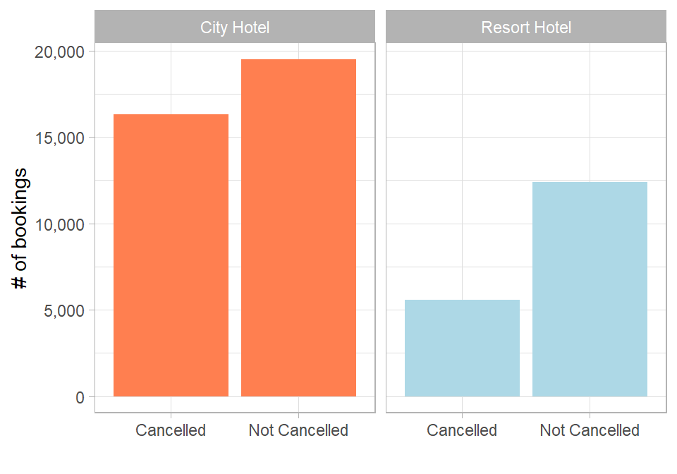
Since our variable of interest is hotel cancellations, a logical starting point is to compare the number of cancelled and non-cancelled bookings across the two hotels:
# Plotting distribution of booking cancellations across hotel typeshotel_cancellations %>%ggplot(aes(x = Is_Cancelled,fill = Hotel)) +geom_bar(show.legend =FALSE) +scale_fill_manual(values =c("#ff7f50", "lightblue")) +scale_y_continuous(labels =comma_format()) +labs(x ="",y ="# of bookings") +facet_wrap(. ~ Hotel)
Figure 26.2: Booking cancellations by hotel type.
The City Hotel has more bookings overall, but also a higher proportion of cancellations. This is visible in the smaller gap between cancelled and non-cancelled bookings compared to the Resort Hotel.
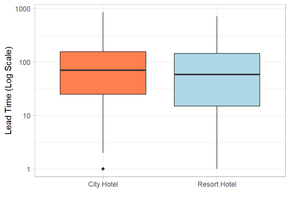
A possible explanation is that resort bookings are more planned, while city hotel bookings may be more flexible or last-minute. To explore this further, we look at lead time—the number of days between booking and arrival—and how it differs across hotels. We use a boxplot with a log scale, since lead time can vary substantially and the log transformation helps reduce skewness and improve comparability. Observations with lead time equal to 0 are excluded, as the logarithm of 0 is undefined:
# Plotting lead time distribution per hotelhotel_cancellations %>%filter(Days_Confirmed_Before_Arrival >0) %>%ggplot(aes(x = Hotel,y = Days_Confirmed_Before_Arrival, fill = Hotel)) +geom_boxplot(show.legend =FALSE) +scale_fill_manual(values =c("#ff7f50", "lightblue")) +scale_y_log10() +labs(x ="", y ="Lead Time (Log Scale)")
Figure 26.3: Lead time distribution by hotel type.
The distribution for the City Hotel appears slightly higher, suggesting longer lead times on average. We can formally assess this difference using a simple linear model. Note that we exclude the observations where Days_Confirmed_Before_Arrival below or equal to 0:
# Fitting linear regression model for testing difference in lead timelm(formula =log(Days_Confirmed_Before_Arrival) ~ Hotel, data = hotel_cancellations %>%filter(Days_Confirmed_Before_Arrival >0) ) %>%summary()
Call:
lm(formula = log(Days_Confirmed_Before_Arrival) ~ Hotel, data = hotel_cancellations %>%
    filter(Days_Confirmed_Before_Arrival > 0))

Residuals:
    Min      1Q  Median      3Q     Max
-3.9734 -0.8379  0.3171  1.1286  2.8803

Coefficients:
                   Estimate Std. Error t value Pr(>|t|)
(Intercept)        3.973367   0.008004  496.44   <2e-16 ***
HotelResort Hotel -0.289782   0.014103  -20.55   <2e-16 ***
---
Signif. codes:  0 '***' 0.001 '**' 0.01 '*' 0.05 '.' 0.1 ' ' 1

Residual standard error: 1.478 on 50331 degrees of freedom
Multiple R-squared:  0.008319,  Adjusted R-squared:  0.008299
F-statistic: 422.2 on 1 and 50331 DF,  p-value: < 2.2e-16
The estimated coefficient for the Resort Hotel is approximately −0.29 and statistically significantly different from 0 at the 1% significance level. Since the dependent variable is in log scale, this implies that lead times for the Resort Hotel are roughly 29% lower on average compared to the City Hotel.
Practical vs Statistical Significance in EDA
This example shows that during EDA, it is not always necessary to fully formalize a statistical model. While checking assumptions and conducting formal inference can strengthen conclusions, simple models and visual patterns are often sufficient to guide intuition. In many business settings, practical relevance is more important than strict statistical significance.
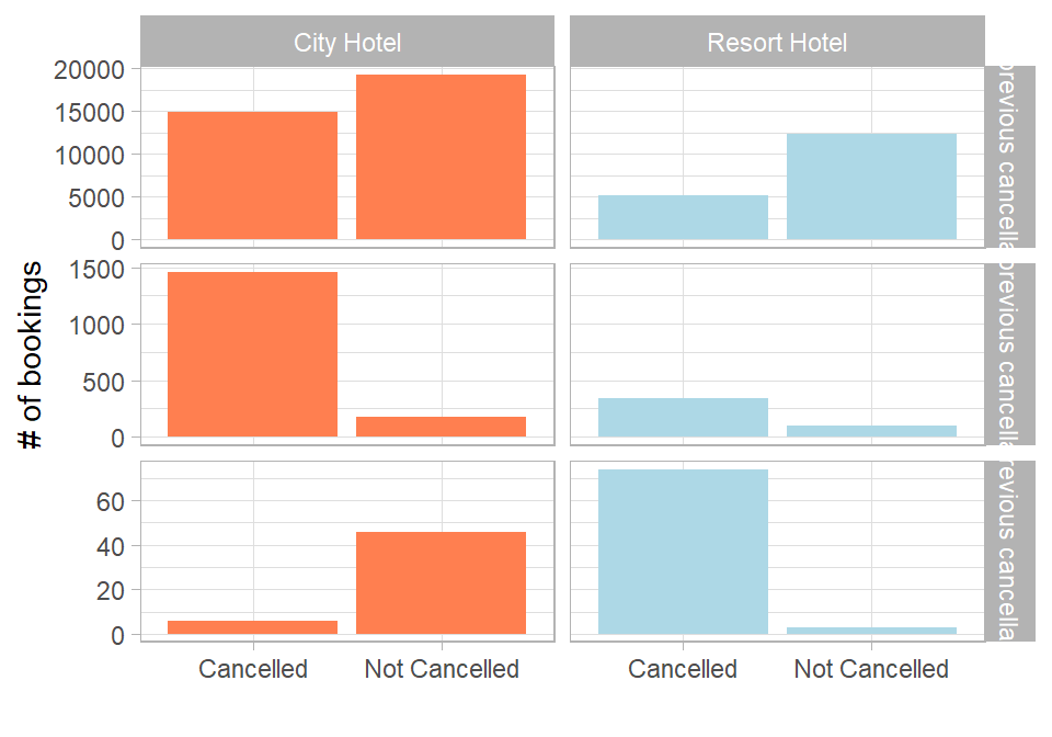
Another factor that may be associated with cancellations is the customer’s past behavior. In particular, if a customer has cancelled bookings before, is it more likely that they will cancel again? To explore this, we examine the number of previous cancellations per customer.
To make this variable easier to interpret, we group customers into three categories based on their cancellation history. The first group includes customers with no previous cancellations, representing customers with no observed history of cancelling bookings. The second group captures customers with a low to moderate cancellation history (1–3 previous cancellations), which may indicate occasional but not systematic cancellation behaviour. Finally, the third group includes customers with a high cancellation history (4 or more previous cancellations), representing customers with a more persistent pattern of cancellations.
Figure 26.4: Cancellations by previous cancellation history and hotel type.
This plot illustrates several interesting insights. First, the majority of bookings with no prior cancellations were not cancelled in either hotel type, with the cancellation rate remaining below 50% in both cases. However, this pattern changes for customers with 1–3 previous cancellations and those with 4 or more cancellations in the resort hotel, where most bookings in both groups were cancelled. Interestingly, the city hotel shows a different pattern: even among customers with 4+ previous cancellations, the majority of bookings were still not cancelled.
To better understand this unexpected pattern, we take a closer look at the actual composition of bookings for customers with at least four prior cancellations by separating previous cancelled and non-cancelled bookings:
The results show that several customers have both many cancellations and many completed stays. At the same time, there are extreme cases, such as a customer with 13 cancellations and no completed stays. These may reflect specific booking behaviors or operational processes (e.g., rebooking at the hotel to modify a reservation). From the data alone, we cannot draw firm conclusions for these cases.
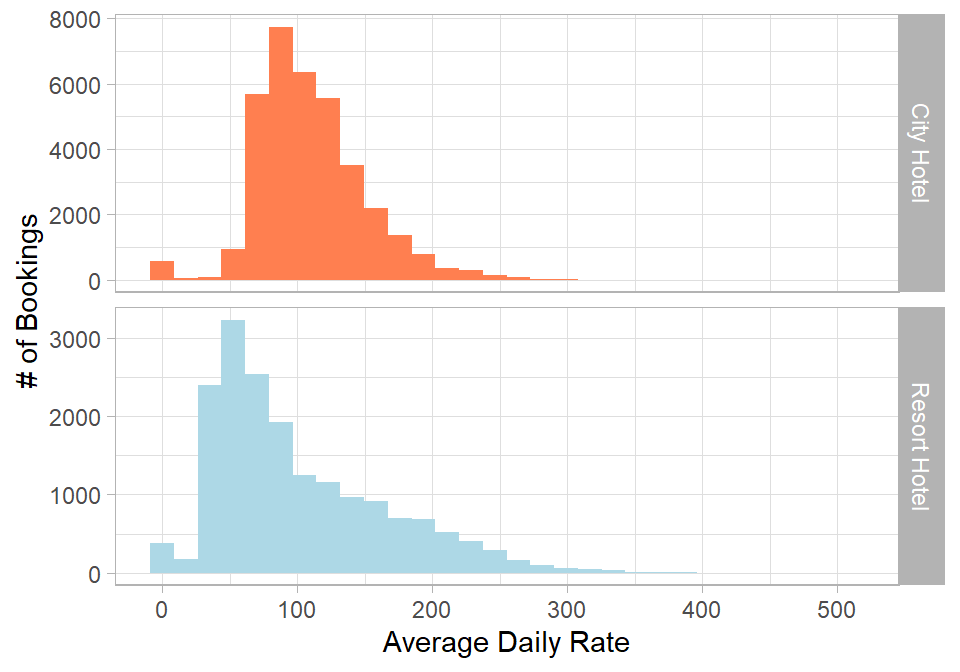
We now turn to pricing by examining the average daily rate (Adr) across the two hotels:
# Plotting distribution of average daily rate (Adr) by hotelhotel_cancellations %>%ggplot(aes(x = Adr, fill = Hotel)) +geom_histogram(show.legend =FALSE) +scale_fill_manual(values =c("#ff7f50", "lightblue")) +facet_grid(Hotel ~ .,scales ="free_y") +labs(x ="Average Daily Rate",y ="# of Bookings")
Figure 26.5: Distribution of average daily rate by hotel type.
This plot reveals three main points. Firstly, the distribution for the City Hotel appears more symmetric, while the Resort Hotel shows a longer right tail. Secondly, both hotels include bookings with an average daily rate of 0. These may reflect data entry issues, promotional stays, or placeholder values. Thirdly, excluding zero values, the City Hotel appears to have higher prices on average, which may not be immediately expected. Given the skewness, it is useful to compare both the mean and the median of Adr for each hotel after removing the zero values.
# Calculating mean and median of Adr per hotel (excluding zero values)hotel_cancellations %>%filter(Adr >0) %>%group_by(Hotel) %>%summarise(Mean_Adr =mean(Adr),Median_Adr =median(Adr))
# A tibble: 2 × 3
  Hotel        Mean_Adr Median_Adr
  <chr>           <dbl>      <dbl>
1 City Hotel       112.        105
2 Resort Hotel     103.         82
Both the mean and the median Adr are higher for the City Hotel than for the Resort Hotel. While this suggests that the City Hotel has higher observed rates in this dataset on average, there are likely additional factors influencing this result. In the hotel industry, prices vary across room types, with larger or higher-quality rooms typically commanding higher rates. To explore this further, we can examine how the average daily rate differs across room types for both hotels. Since there are many room categories, we use the function fct_lump() to group those with relatively few observations into a single category labeled Other:
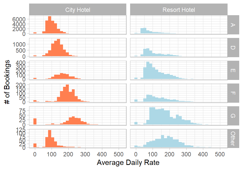
# Plotting Adr across reserved room types by hotelhotel_cancellations %>%mutate(Reserved_Room_Type =fct_lump(Reserved_Room_Type, n =4)) %>%ggplot(aes(x = Adr, fill = Hotel)) +geom_histogram(show.legend =FALSE) +scale_fill_manual(values =c("#ff7f50", "lightblue")) +facet_grid(Reserved_Room_Type ~ Hotel, scales ="free_y") +labs(x ="Average Daily Rate", y ="# of Bookings")
Figure 26.6: Distribution of average daily rate by reserved room type and hotel.
For both hotels, higher room categories tend to shift the distribution to the right, indicating higher prices. The City Hotel distributions remain relatively symmetric, while the Resort Hotel distributions are more positively skewed. Zero values appear across all room types, reinforcing the earlier observation. To better understand these zero values, we count how often they occur:
# Counting zero Adr values by hotel and cancellation statushotel_cancellations %>%mutate(Zero_Adr =if_else(Adr ==0, 1, 0)) %>%group_by(Hotel, Is_Cancelled) %>%summarize(Total_Zero_Adr =sum(Zero_Adr)) %>%ungroup()
# A tibble: 4 × 3
  Hotel        Is_Cancelled  Total_Zero_Adr
  <chr>        <chr>                  <dbl>
1 City Hotel   Cancelled                 64
2 City Hotel   Not Cancelled            479
3 Resort Hotel Cancelled                 32
4 Resort Hotel Not Cancelled            302
The results show that a value of 0 does not necessarily imply a cancellation. In most cases, these bookings are not cancelled, suggesting that at least some of them may correspond to promotional or special cases. Although these observations appear unusual, their frequency suggests that they are not purely data entry errors.
Iterative Nature of Data Analysis
We might find that these zero values are not valid observations and decide to remove them. This would mean going back to the data cleaning step, removing these values, and potentially re-creating the subsequent plots. This highlights a common misconception that data analysis is a linear process—in practice, it is often iterative, with earlier steps being revised as new insights emerge.
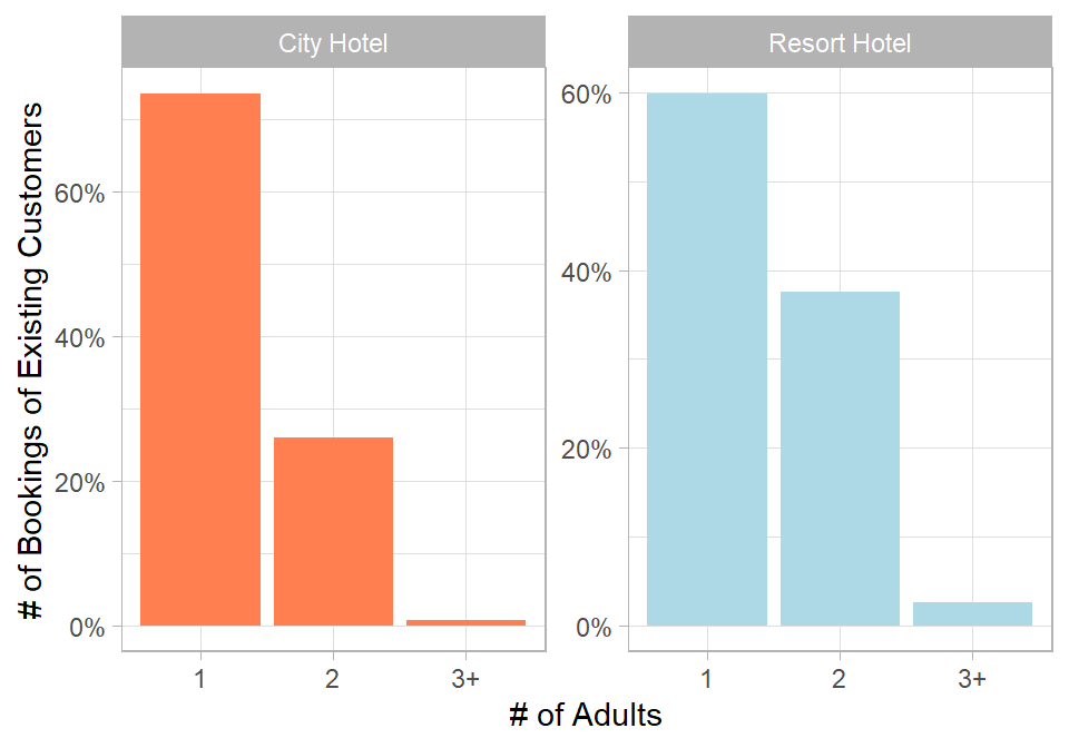
To conclude the exploratory analysis, we examine how bookings from existing customers vary by the number of adults:
# Plotting distribution of existing customer bookings by number of adults and hotelhotel_cancellations %>%filter(Customer_Type =="Existing Customer"& Adults >0) %>%mutate(Adults =case_when( Adults ==1~"1", Adults ==2~"2",TRUE~"3+")) %>%count(Hotel, Adults) %>%group_by(Hotel) %>%mutate(n = n/sum(n)) %>%ggplot(aes(x = Adults,y = n,fill = Hotel)) +geom_col(show.legend =FALSE) +scale_fill_manual(values =c("#ff7f50", "lightblue")) +facet_wrap(. ~ Hotel,scales ="free_y") +labs(x ="# of Adults", y ="Booking Share (%)") +scale_y_continuous(labels =percent_format())
Figure 26.7: Distribution of existing customer bookings by number of adults and hotel type.
In both hotels, most bookings from existing customers are for 1 adult. However, about 40% of existing customer bookings at the Resort hotel involve at least 2 adults, compared to nearly 30% at the City hotel. This may suggest that returning guests at the Resort hotel are more likely to travel with companions, possibly for vacations or family trips.
Overall, these findings give some useful insights for hotel management. First, the City Hotel shows higher cancellation rates compared to the Resort Hotel, which suggests that cancellations behave differently across the two settings. In practice, this could require targeted strategies such as stricter booking policies, deposits, or incentives to reduce cancellations and improve booking reliability. Additionally, past customer behavior—especially previous cancellations—clearly seems related to future cancellations. This information can be used for better segmentation of customers and for improving forecasting models, since some groups of customers are more likely to cancel than others. Also, pricing patterns differ across hotels and room types. This indicates that differences in revenue are not only driven by the hotel itself, but also by the composition of room types and demand structure. This can be useful for more detailed revenue management and pricing decisions. Finally, the zero values in variables such as Adr should be treated carefully. In practice, these values should ideally be checked and clarified with the data provider, since they may represent missing values, special cases, or recording issues. Ignoring them without investigation could lead to misleading summaries and affect the overall interpretation of the results.
Predictive Modeling
The exploratory data analysis helped us uncover key patterns and behaviors in the hotel booking data, shedding light on how factors such as booking lead time, duration of stay, previous customer behavior, and booking changes relate to the likelihood of cancellation. These insights are already useful for hotel managers in making more informed decisions, although so far they do not provide exact quantitative predictions.
Even though these insights were valuable for understanding factors associated with cancellations, we can go one step further. From a data science perspective, it is useful to investigate whether we can build a predictive model that can estimate the probability of a booking being cancelled before it actually happens. Regarding the suspicious observations, such as Adr values equal to 0 or bookings with 0 adults and children, we keep these observations for now, mainly because they are not directly linked to only cancelled or non-cancelled bookings. However, in practice, these issues should be communicated before any predictive modeling, to ensure the validity of both the data and the results.
In the context of hotel cancellations, a predictive model could provide real-time cancellation risk scores for incoming bookings. This would allow hotels to take proactive actions, such as overbooking strategies, targeted communication, or policy adjustments, in order to reduce the negative impact of cancellations. Assuming no major shifts in customer behavior, this transforms the patterns identified in the exploratory analysis into actionable predictions, adding direct business value beyond descriptive insights.
Before building any model, it is important to clarify the problem setup. This is a binary classification problem, meaning the target variable has two possible outcomes: cancellation or no cancellation. In other words, we are trying to classify expected customer behavior. Based on this, we can define four possible outcomes:
Correctly predict that a booking will be cancelled (True Positive, TP)
Incorrectly predict that a booking will be cancelled (False Positive, FP)
Correctly predict that a booking will not be cancelled (True Negative, TN)
Incorrectly predict that a booking will not be cancelled (False Negative, FN)
These are the standard outcomes as discussed Chapter Model Validation and Performance Evaluation. From a machine learning perspective, we are particularly interested in the metrics precision and recall. In this context, precision measures how many of the predicted cancellations are actually correct, while recall measures how many of the actual cancellations we are able to correctly identify.
In practice, such a dataset would normally include a timestamp indicating when a booking was made or cancelled. Since we do not have this information, we treat the dataset as cross-sectional, assuming that each row is independent of the others. Therefore, to evaluate model performance, we can use resampling methods such as k-fold cross-validation. At the beginning, we also keep a small portion of the data as a hold-out (test) set for final evaluation.
Regarding machine learning methods, we will apply KNN, Naive Bayes, and random forest. We do not include decision trees or bagged trees separately, as we will use random forest as a tree-based method. Linear regression is also excluded, since it is mainly used for regression problems rather than classification.
Note on Logistic Regression
It would also be possible to use the linear regression counterpart for binary classification problems, known as logistic regression. Since this method was not covered in the book, however, we will skip it here. As always, it is recommended to use only methods that are familiar at this stage.
Let’s start by loading the tidymodels package, setting tidymodels_prefer(), and splitting hotel_cancellations into training and test sets using an 80/20 split. We also create 5-fold cross-validation folds based on the training set. A stratified sampling approach is used to ensure that the proportion of cancellations is similar in both the training and test data, as well as across the folds. We also transform the variable Is_Cancelled from a character into a factor, as this is required in tidymodels for classification tasks. It is also worth noting that tidymodels requires the discrim package in order to implement Naive Bayes via the naive_bayes engine.
# Librarieslibrary(tidymodels)library(discrim)# Ensuring tidymodels functions prioritytidymodels_prefer()# Setting seedset.seed(999)# Training and test setshotel_cancellations <- hotel_cancellations %>%mutate(Is_Cancelled =factor(x = Is_Cancelled, levels =c("Cancelled", "Not Cancelled")) )# Setting seedset.seed(999)# Splitting customer_churnsplit_data <-initial_split( hotel_cancellations, prop =0.8, strata = Is_Cancelled)# Extracting the training settraining_set <- split_data %>%training()# Extracting the test settest_set <- split_data %>%testing()# 5 cross-validation foldsfolds_cv <-vfold_cv(training_set, v =5)
Next, we initiate the model engines for random forest, KNN, and Naive Bayes. For random forest, we will tune the hyperparameters mtry and min_n, which control the number of predictors considered at each split and the minimum number of observations required in a node, respectively. For KNN, we tune the number of neighbors (neighbors), which determines how many nearby observations are used to classify a new point. For Naive Bayes, we set the laplace argument to 1 to apply Laplace smoothing. This is done to avoid zero probabilities when a category is not observed in the training data, ensuring that the model remains stable and can make predictions even for previously unseen combinations.
The next step is to create a recipe for each method. We include all available variables, as they may all carry predictive information about the target variable, even if some of them were not analyzed in detail during the exploratory phase. This helps ensure that potentially relevant signal is not prematurely excluded from the model, especially in machine learning settings where interactions and nonlinear effects may be captured automatically. Random forest does not require any preprocessing such as standardizing predictors, so we only define the formula within the recipe. For KNN, we create dummy variables for all categorical predictors using step_dummy() together with all_nominal_predictors(), which selects all nominal (categorical) variables. This is necessary because KNN relies on distance calculations, which require all predictors to be in a numeric format. In contrast, Naive Bayes handles categorical predictors naturally, but it cannot directly handle continuous numeric variables in their raw form. For this reason, we apply step_discretize() to numeric predictors, converting them into a small number of categories. In this case, we split each numeric variable into three groups. For example, Adr is transformed into three categories representing low, medium, and high values based on its distribution.
# Random forest - Reciperf_recipe <-recipe(Is_Cancelled ~ ., data = training_set)# KNN - Recipeknn_recipe <-recipe(Is_Cancelled ~ ., data = training_set) %>%step_dummy(all_nominal_predictors()) %>%step_normalize(all_numeric_predictors())# Naive Bayes - Recipenb_recipe <-recipe(Is_Cancelled ~ ., data = training_set) %>%step_discretize(all_numeric_predictors(), num_breaks =3)
Now we can combine each model with its corresponding recipe to create three different workflows, one for each method:
Before fitting any model, it is necessary to specify the hyperparameter values we want to test. As discussed in Chapter Hyperparameter Tuning, we create a tibble where the column names correspond to the hyperparameters and the rows define the values we want to evaluate.
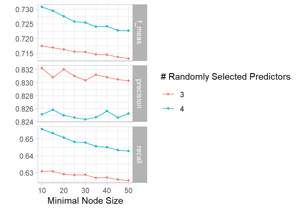
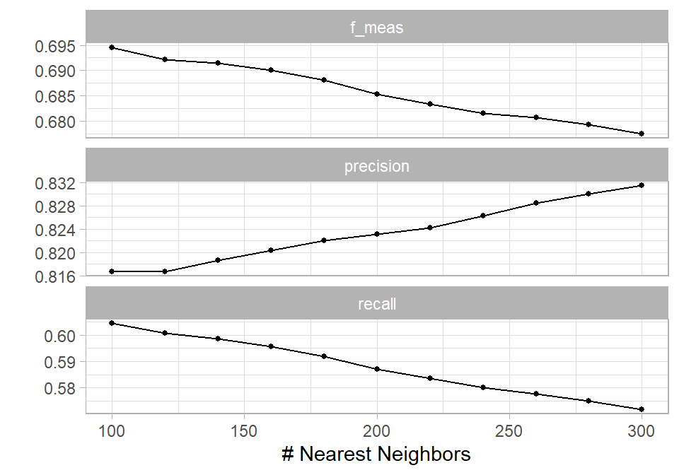
For random forest, we choose values 3 and 4 for mtry, and values from 10 to 50 in steps of 5 for min_n. Since we want to evaluate all possible combinations of these values, we use the function crossing(), which generates a grid of all combinations between the provided inputs (i.e., every value of mtry is paired with every value of min_n). For KNN, we define the number of neighbors as a sequence from 100 to 300 in steps of 20. This controls how many nearby observations are used when making predictions, with larger values producing smoother but less flexible models. Naive Bayes does not require hyperparameter tuning in this setup, so no grid is specified for this method:
# Random Forest - Gridrf_grid <-crossing(min_n =seq(from =10, to =50, by =5),mtry =3:4 )# KNN - Gridknn_grid <-tibble(neighbors =seq(from =100, to =300, by =20) )
We can now apply cross-validation to all models. Because we perform hyperparameter tuning for random forest and KNN, we use the function tune_grid() together with the corresponding grid tibbles. For Naive Bayes, we use fit_resamples(), since there are no hyperparameters to tune and we only evaluate the model across the resamples.
For the evaluation metrics, as mentioned earlier, we are mainly interested in precision and recall. Therefore, we include these metrics using the metric_set() function. In addition, we also include the F1-score (f_meas), since it combines precision and recall into a single measure and provides a balanced view of model performance when both types of errors are important:
The results are quite informative. For random forest, precision is higher when mtry = 3, while recall and F1-score are higher when mtry = 4. In addition, across both values of mtry, performance generally improves when the minimum node size (min_n) is smaller. Based on this, we select the model with mtry = 4 and min_n = 10 as the best overall configuration. This model also performs better than all KNN alternatives, where the best results are obtained with the smallest number of neighbors (100). Overall, KNN shows weaker performance compared to tree-based methods in this setting.
For Naive Bayes, since there are no hyperparameters, we directly inspect the average cross-validation results. The model achieves very high precision (close to 100%), but relatively low recall (approximately 37%). This means that when the model predicts a cancellation, it is almost always correct, but it only identifies a limited proportion of all actual cancellations.
Based on the F1-score, random forest is the best overall model for this problem. However, if precision is the main priority, Naive Bayes can still be a useful starting point, especially in early stages where predictive systems are not yet implemented. As discussed earlier in this chapter, when starting from scratch, it is usually advisable to first run a small-scale experiment and gradually move toward more complex decision systems.
Ultimately, the choice between random forest and Naive Bayes depends on the business context, the cost of false positives versus false negatives. In practice, this is not only a technical decision but also a strategic one, as different stakeholders may value different types of errors differently. However, only for illustrating purposes (and to satisfy any curiosity) we proceed with both models to see how they perform on the test set.
For random forest, we need to select the best hyperparameters for random forest as discussed, finalize the workflow and use the last_fit() function:
# Random forest - Selecting best parametersrf_best_params <- rf_results %>%select_best(metric ="f_meas")# Random forest - Finalizing workflowrf_final_workflow <-finalize_workflow(x = rf_workflow, parameters = rf_best_params)# Random forest - Fitting the model on the training set and evaluating it on the test setrf_final_fit <-last_fit(object = rf_final_workflow,split = split_data, metrics =metric_set(precision, recall, f_meas))# Collecting metricscollect_metrics(rf_final_fit)
The test set results are very close to the cross-validation results, which suggests that the model generalizes well and that the validation process was reliable.
Because Naive Bayes had no hyperparameters, we do not need to finalize the workflow. For symmetry though, we create another object called nb_final_workflow, in which we simply assign the nb_workflow object. We then proceed with last_fit() as we did earlier:
# Naive Bayes - Selecting best parametersnb_best_params <- nb_results %>%select_best(metric ="f_meas")# Naive Bayes - Finalizing workflownb_final_workflow <- nb_workflow# Naive Bayes - Fitting the model on the training set and evaluating it on the test setnb_final_fit <-last_fit(object = nb_final_workflow,split = split_data, metrics =metric_set(precision, recall, f_meas))# Collecting metricscollect_metrics(nb_final_fit)
Similarly, Naive Bayes shows very consistent performance between cross-validation and the test set, confirming that the model behaves as it should on previously unseen data.
Overall, this comparison highlights an important lesson: there is no universally best model. In practice, the best model depends on the specific goal of the problem and the cost of different types of errors. This once again illustrates the idea behind the No Free Lunch theorem in machine learning, where no single model performs best across all problems.
Closing
This chapter concludes with a case study that included most of the methods we discussed throughout this book. I hope this book has been of value to you and that you have gained a solid understanding of the core concepts and workflows in data science and machine learning. More importantly, I hope you enjoyed this journey, even if you do not see yourself as a future data scientist.
Data is everywhere, and I strongly believe that data science is more than just a profession: it is a way of logical and critical thinking. Especially in the business world, the most important skill is how to approach a problem in a structured way and translate it into a data-driven solution. At this point, you are already equipped with more than enough tools to do so.
Remember, data science is as much an art as it is a science, requiring both technical methods and thoughtful interpretation. The real value comes not only from building models, but also from asking the right questions, making reasonable assumptions, and communicating results in a clear and meaningful way.