Hierarchical Clustering
Introduction
In this chapter, we explore hierarchical clustering, a widely used method for uncovering natural groupings in data. Compared to k-means clustering, hierarchical clustering is often easier to understand and implement. It does not require the number of clusters to be specified in advance and instead produces a tree-like diagram known as a dendrogram, which illustrates how observations are grouped together at various levels of similarity.
One of the key advantages of hierarchical clustering is its flexibility: the dendrogram reveals all possible clusterings, from the finest level—where each observation is its own cluster—to the broadest level—where all observations are merged into one. The user can then choose the number of clusters by “cutting” the dendrogram at a specific height.
There are two main types of hierarchical clustering: bottom-up (agglomerative) and top-down (divisive). We focus on the bottom-up approach, which begins by treating each observation as its own cluster and then successively merges the closest pairs of clusters based on a defined distance metric, gradually building a hierarchical structure.
Hierarchical Clustering in Depth
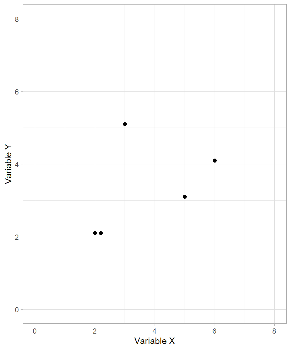
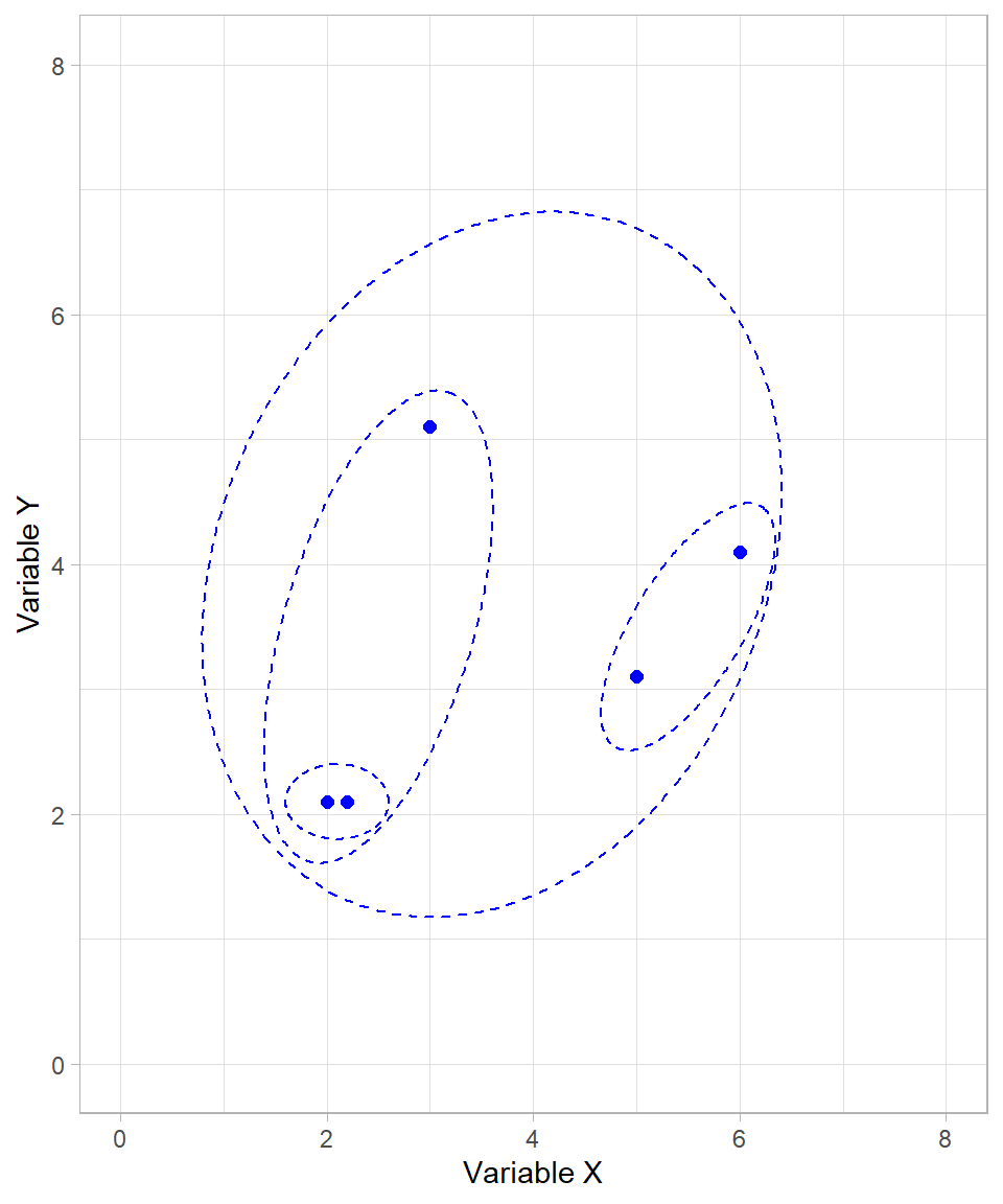
To start, let’s examine the following fictional example. Suppose we want to create clusters for the following observations based on two variables, \(X\) and \(Y\):
The process of hierarchical clustering works as follows: we measure the distances between each pair of data points and cluster together the ones that are closest. As with k-means clustering, we usually use the Euclidean distance formula. Scaling the variables is also an important step, but we skip it in this fictional example for simplicity.
In the plot above, it is clear that the two points on the bottom left are closer to each other. These two points then form the first cluster:
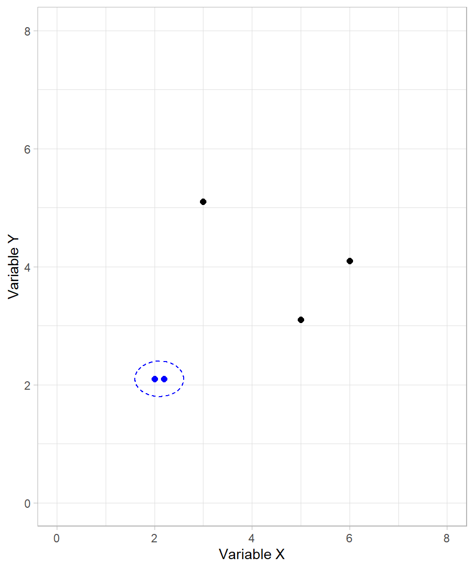
After creating the first cluster, the algorithm continues by recalculating distances. For already clustered data points, their cluster as a whole is considered. We’ll discuss the precise rules for this later. For now, it suffices to understand that the formed cluster behaves like a single data point.
In our example, the next cluster formed includes the two data points on the right-hand side of the plot:
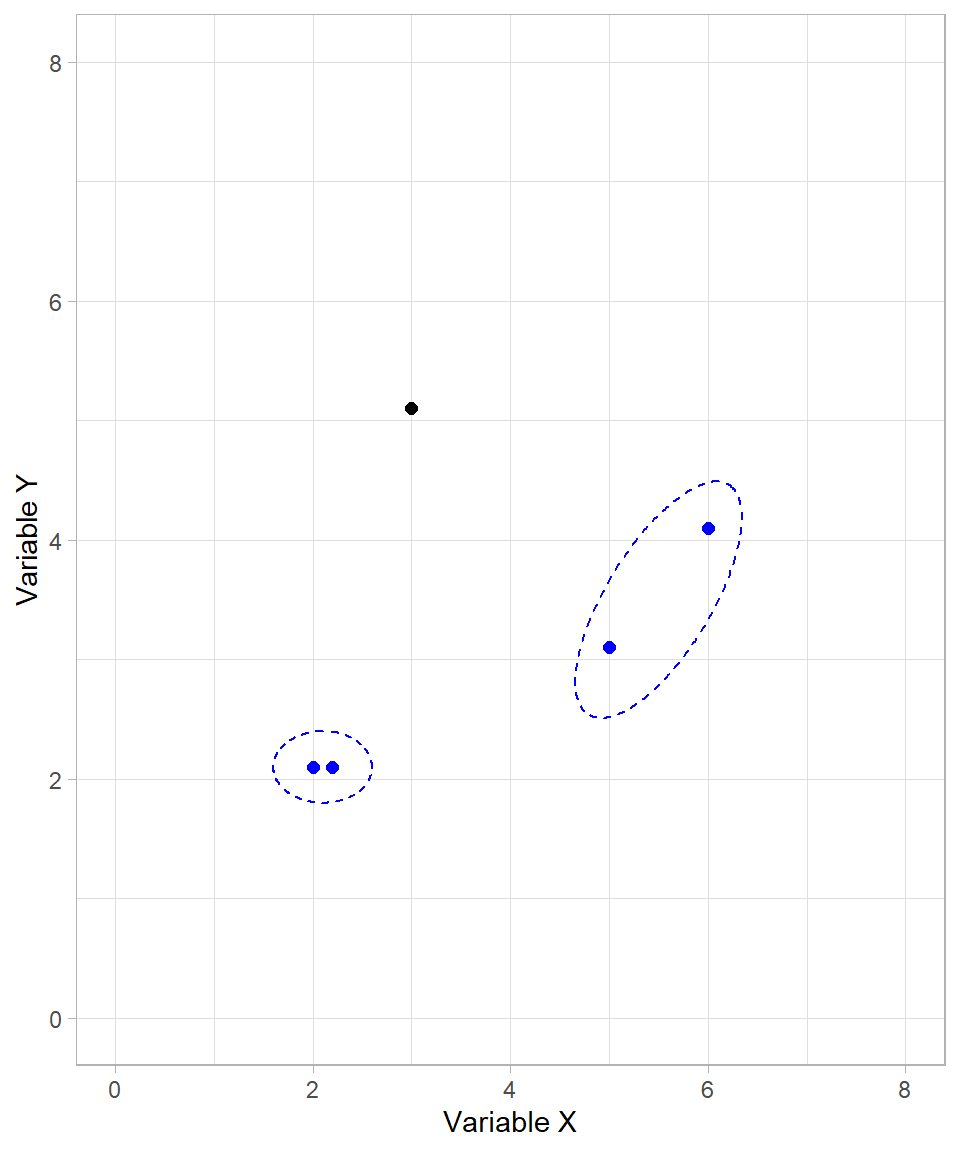
We now have two formed clusters and one unclustered data point. The algorithm proceeds by joining the unclustered point with the first cluster:
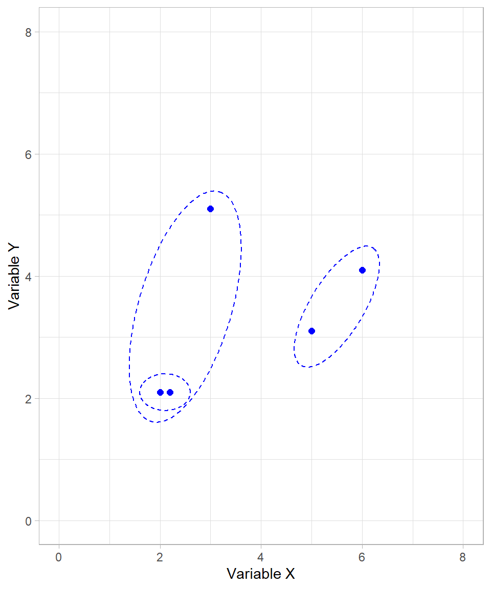
Although all data points are now in clusters, the algorithm continues until only one cluster remains. The final merge step combines the two large clusters into one:
Our algorithm has now finished. All possible clusters have been created, starting from the smallest possible (individual data points) to the largest possible (a single cluster with all data points).
Because we started with the individual data points and then formed clusters on a higher and higher level, we call this type bottom-up (or agglomerate). The alternative would be a top-down (or divisive) approach, which starts with all observations in a single cluster and recursively splits them into smaller clusters. Divisive clustering is less commonly used than agglomerative clustering, mainly because it is computationally intensive, but it can be useful in certain cases where the overall structure of the data is better captured by successive splits rather than successive merges. This may seem similar to tree-based models (see Chapter Tree-Based Models), where each subsequent node represents a split in the data based on a particular criterion. However, the key difference is that divisive clustering is unsupervised and relies purely on distances or dissimilarities between observations, while tree-based models are supervised and split data according to a target variable to optimize prediction accuracy.
Dendrogram
The sequence of clustering steps we just visualized—starting from individual points and merging them based on proximity—forms the foundation of the dendrogram, the key output of hierarchical clustering. This tree-like structure records each step of the clustering process. Observations that are more similar to each other are merged earlier (at lower heights), while more distinct groupings merge later (at greater heights).
One of the main strengths of the dendrogram is its applicability to datasets with more than two variables. While scatter plots work well for two-dimensional data, they quickly become impractical in higher dimensions. In such cases, the dendrogram provides a clear and interpretable summary of the clustering process, allowing us to examine the relationships between observations and clusters without relying on geometric intuition.
The dendrogram of our example earlier is the following:
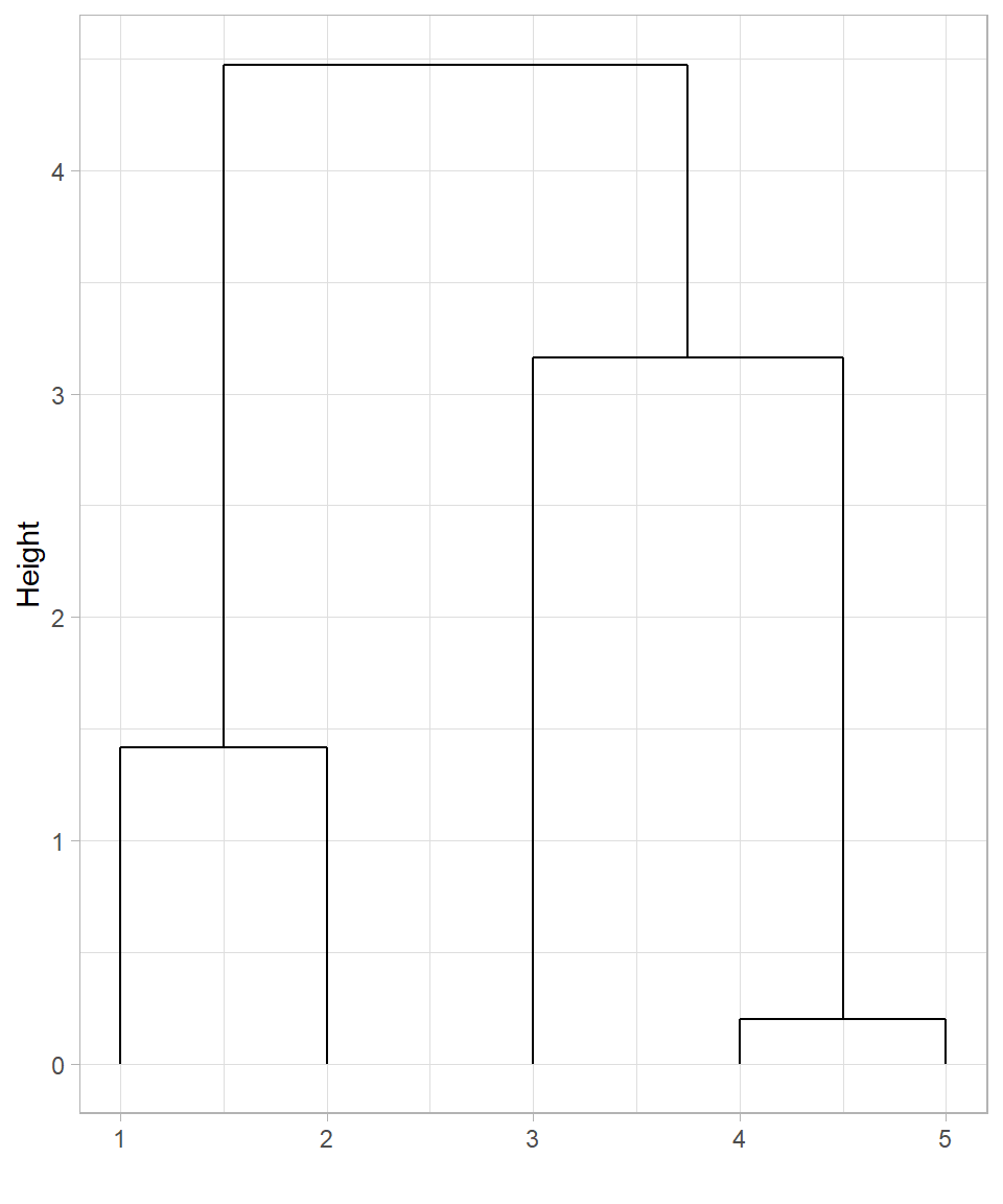
In this dendrogram:
The horizontal axis displays the indices of the observations (row numbers).
The vertical axis shows the height at which clusters are merged, which corresponds to the distance between the clusters at the time of merging.
This dendrogram represents the same sequence of merges we illustrated visually:
The first cluster combines observations 1 and 2 (the closest pair).
Next, observations 3 and 4 are merged.
Then, observation 5 joins the cluster formed by points 1 and 2.
Finally, all observations are merged into one cluster at the highest level.
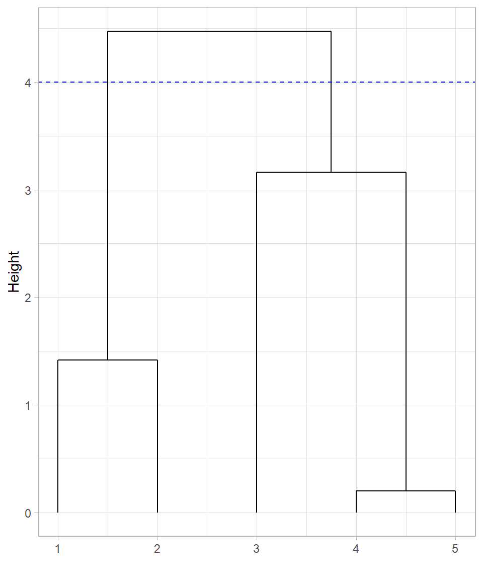
The dendrogram not only shows how the clusters were formed, but also provides a tool for choosing the number of clusters. Drawing a horizontal line across the dendrogram at a particular height effectively cuts the tree at that point. The vertical branches intersected by this cut correspond to the clusters at that level of dissimilarity.
For example, if we draw a horizontal line near the middle of the dendrogram, we may obtain three clusters. A lower cut may produce more (but smaller) clusters, while a higher cut yields fewer (yet larger) clusters.
Cutting the tree at height 4 produces 2 clusters, as there are two lines at that height. In this case, observations 1 and 2 would belong in the first cluster while the rest would belong in the second cluster:
What if we decide to cut the tree at height 2 instead of height 4?
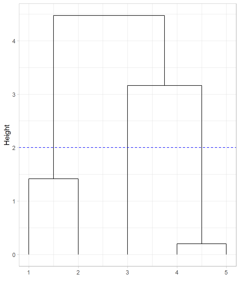
Cutting the tree at height 2 would create three clusters, with data point 3 appearing not yet merged into any cluster at that height. However, it’s important to clarify that data point 3 is not truly unclustered—in hierarchical clustering, all observations are always part of the hierarchy. What happens instead is that cutting at a lower height isolates data points into their own individual clusters. So, at height 2, data point 3 forms a singleton cluster, while points 1 and 2, and points 4 and 5, form the other two clusters.
This illustrates the flexibility of hierarchical clustering: we can adjust the level of granularity in our clustering results by choosing different cut heights.
The dendrogram, therefore, not only records the full clustering process but also gives us control over the final clustering structure by allowing us to “cut” the tree at a level that suits our analytical needs.
Determining the Distance of a Cluster
Calculating the distance between two individual data points is straightforward using standard distance measures such as Euclidean distance. However, hierarchical clustering quickly faces a more complex question: how do we compute the distance between a cluster (which may contain multiple data points) and another point or cluster?
This decision is critical because it directly affects how clusters are formed and ultimately determines the shape of the resulting dendrogram.
Let’s revisit our visual example where two clusters are formed, but this time there also an extra data point that represents the center of one of the created clusters:
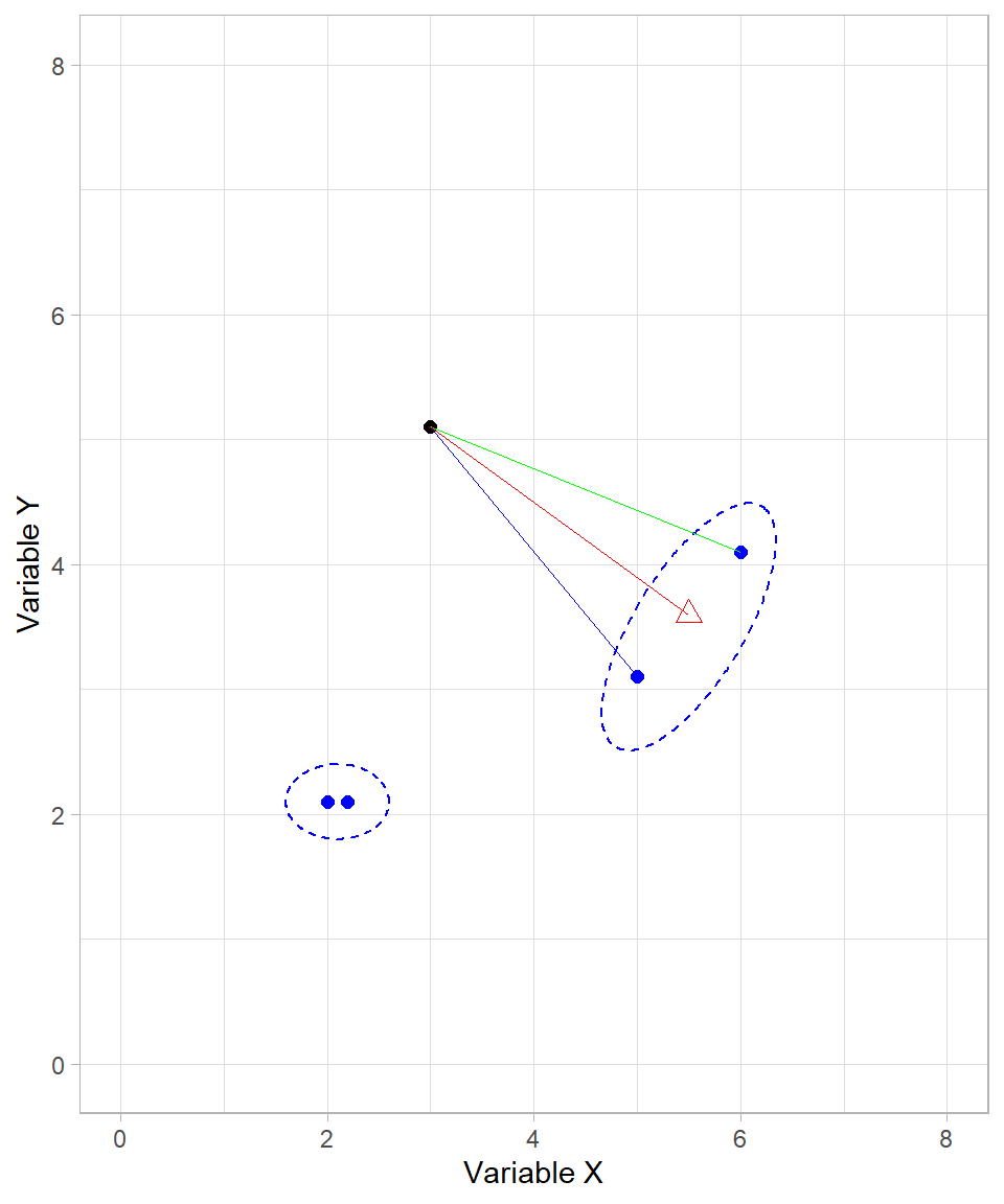
When one or both of the objects being compared are clusters (i.e., sets of data points), we must decide how to measure the distance between them. Several methods exist, each with a different interpretation:
Single linkage: The distance between the two closest points in each cluster (blue line).
Complete linkage: The distance between the two furthest points in each cluster (green line).
Centroid linkage: The distance between the centroids (geometric centers) of the two clusters (red line).
Average linkage: The average distance between all pairs of points across the two clusters (not shown explicitly in the plot, but conceptually intermediate between single and complete linkage).
These are known as linkage methods, because they define how clusters are “linked” during the merging process. Each linkage method may yield a different clustering result, even on the same dataset. For example, single linkage often produces elongated, chain-like clusters, while complete linkage tends to form compact, spherical clusters. Average and centroid linkage strike a balance between the two extremes.
Among these, complete linkage and average linkage are the most commonly used in practice. They typically produce more balanced dendrograms, which helps in avoiding overly large or overly fragmented clusters. The selection of a linkage method is always made before running the hierarchical clustering algorithm, as it governs how distances are calculated during the iterative merging process.
Assumptions
Hierarchical clustering operates under a set of assumptions that influence its effectiveness and, respectively, the validity of its results. Understanding these assumptions helps us recognize when hierarchical clustering is appropriate—and when it may not be the best choice (Murtagh & Contreras, 2012; Tan et al., 2019).
Hierarchical structure exists: The method assumes that the data can be naturally grouped into nested clusters. That is, small clusters should merge cleanly into larger ones. If the underlying structure is not hierarchical, the method may produce misleading or unstable results. For example, imagine a set of points that are all scattered randomly with no clear groups. In this case, there are no natural clusters to merge, so hierarchical clustering will force groupings that don’t really exist.
Linkage criteria reflect group similarity: The way we define the distance between clusters (via the linkage method) significantly impacts the outcome. The algorithm assumes that the chosen linkage method—such as complete, average, or single—accurately captures how clusters are meant to be formed. Different linkage methods can lead to very different dendrograms and clusters.
Distance metrics are meaningful: Hierarchical clustering also assumes that the chosen distance metric (e.g., Euclidean) appropriately represents similarity among observations. Variables should be scaled if they are on different ranges; otherwise, one variable may dominate the distance calculation and distort clustering results.
These assumptions underscore the importance of combining hierarchical clustering with domain knowledge and visual inspection of the dendrogram (Everitt et al., 2011).
Hierarchical Clustering in R
To apply hierarchical clustering in R, we will work with the dataset website_visits, used also in Chapter K-Means. Since the dataset has already been introduced, we won’t describe it again. Our goal here is to compare how hierarchical clustering organizes the data relative to k-means, which (k-means) formed four clusters.
To start, we load the tidyverse package, import the dataset and standardize the variables Website_Visits and Purchased_Products:
# Libraries
library(tidyverse)

# Importing the dataset
website_visits <- read_csv("https://raw.githubusercontent.com/DataKortex/Data-Sets/refs/heads/main/website_visits.csv")

# Standardize function
standardization <- function(x) {return((x - mean(x)) / sd(x))}

# Applying standardization on the variables
website_visits <- website_visits %>%
  mutate(Website_Visits = standardization(Website_Visits),
         Purchased_Products = standardization(Purchased_Products))
The following scatterplot reflects the standardized data of website_visits:
# Plotting website_visits
website_visits %>%
    ggplot(aes(x = Website_Visits,
               y = Purchased_Products)) +
    geom_point(size = 2,
               color = "skyblue") +
  labs(x = "Website Visits",
     y = "Purchased Products")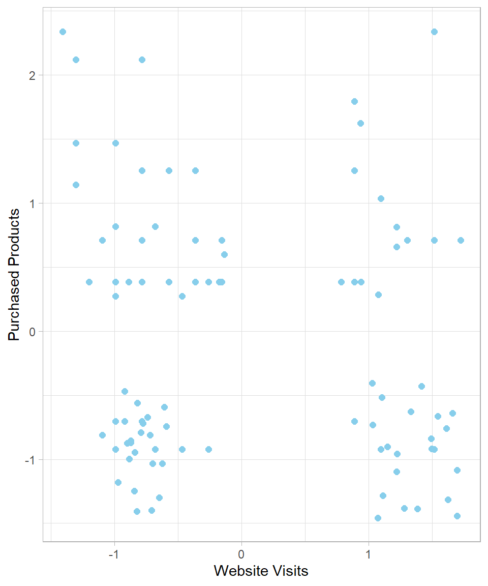
To calculate the distances between data points, we use the function dist(), which returns a distance object. We then apply hierarchical clustering with the function hclust(), passing this distance object as the d argument:
# Calculating distances
website_visits_distances <- dist(x = website_visits)

# Hierarchical clustering
hclust_website_visits_complete <- hclust(d = website_visits_distances)
The default linkage method is complete linkage, but we can choose a different method by specifying the argument method. For example, the following code uses the average linkage method:
# Hierarchical clustering with average linkage
hclust_website_visits_average <- hclust(d = website_visits_distances,
                                        method = "average")
Now we have two different dendrograms—one created using the complete linkage method and the other using the average linkage method. Although base R’s plot() function can display dendrograms, ggplot2 provides more flexible and customizable visualizations. To do this, we first need to transform the hierarchical clustering object into a format that ggplot2 can work with. This is achieved using the function dendro_data() from the ggdendro package. The dendro_data() function takes an hclust object and returns a list containing multiple components, including a data frame called segment. This data frame contains all the information needed to draw the line segments of the dendrogram: the start and end coordinates of each segment, as well as additional labeling information if needed. We can extract this data frame using the $segment operator or by applying the segment() function directly to the list returned by dendro_data().
Once we have this data frame, we can map its columns to aesthetics in ggplot2 using the function geom_segment(). Each row of the data frame corresponds to a line segment in the dendrogram, with x and xend specifying the horizontal positions and y and yend specifying the vertical positions (heights at which clusters merge). By passing these mappings to geom_segment(), we can recreate the dendrogram entirely within the ggplot2 framework, allowing full control over line types, colors, annotations, and integration with other ggplot2 layers.
The following code demonstrates this process for the complete linkage dendrogram:
# Plotting website_visits
# Libraries
library(ggdendro)

# Converting hclust object to dendrogram data
dend_data_complete <- dendro_data(hclust_website_visits_complete)

# Plotting dend_data_complete
dend_data_complete %>%
  segment() %>%
  ggplot() +
  geom_segment(aes(x = x,
                   y = y,
                   xend = xend,
                   yend = yend)) +
  labs(x = "",
       y = "Height")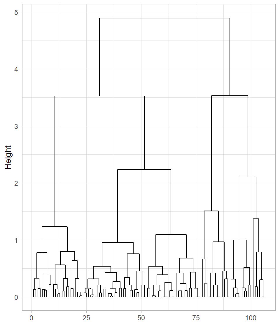
# Converting hclust object to dendrogram data
dend_data_average <- dendro_data(hclust_website_visits_average)

# Plotting dend_data_average
dend_data_average %>%
  segment() %>%
  ggplot() +
  geom_segment(aes(x = x,
                   y = y,
                   xend = xend,
                   yend = yend)) +
  labs(x = "",
       y = "Height")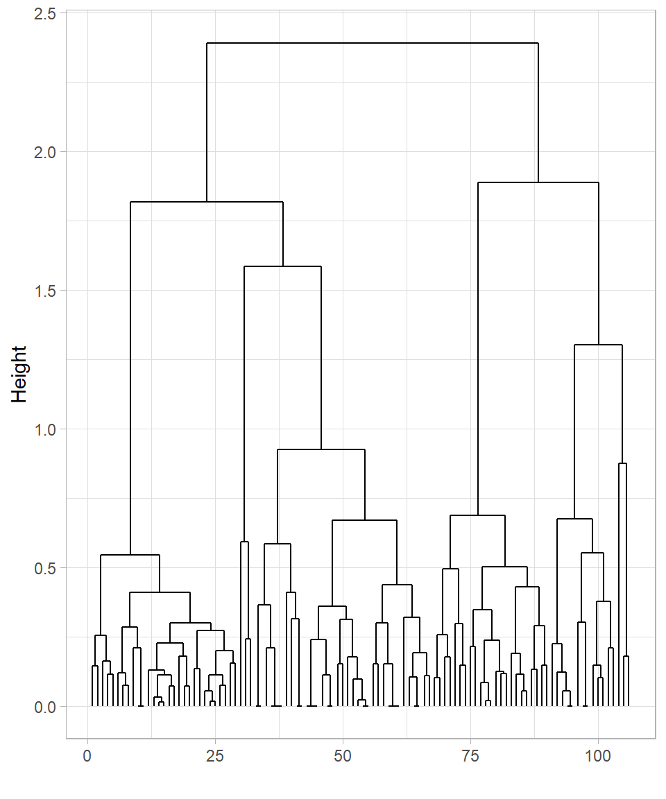
The two dendrograms are similar but still show some differences. In both cases, many observations cluster near the bottom, which makes it difficult to clearly distinguish the formed clusters.
To keep things simple, let’s focus on the dendrogram created using the complete linkage method. It’s apparent that cutting the tree at height 4 would produce two clusters, while cutting at height 3 would result in four clusters. We can visualize these cuts on the dendrogram using the function geom_hline(), which draws horizontal lines on a plot. To specify the height—the value on the y-axis—we set the yintercept argument to the desired value:
# Plotting dend_data_complete with horizontal lines
dend_data_complete %>%
  segment() %>%
  ggplot() +
  geom_segment(aes(x = x,
                   y = y,
                   xend = xend,
                   yend = yend)) +
  labs(x = "",
       y = "Height") +
  geom_hline(yintercept = 4, color = "blue") +
  geom_hline(yintercept = 3, color = "blue")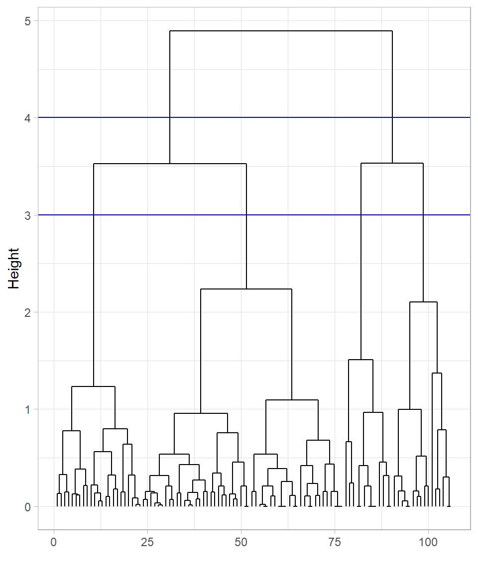
These cuts are only visualized on the plot; the tree itself hasn’t been cut yet. To actually cut the tree, we use the function cutree(), providing the hclust_data_complete object in the argument tree and specifying the cut height with the h argument:
# Cutting the tree at height 3
clusters_height_3 <- cutree(tree = hclust_website_visits_complete, h = 3)

# Printing clusters_height_3
clusters_height_3
[1] 1 1 1 1 2 3 1 1 4 4 1 4 1 4 1 1 1 2 2 2 2 2 1 3 4 1 4 1 1 4 1 1 2 4 1 1 1
[38] 1 4 1 4 1 1 1 1 1 1 1 2 1 2 1 2 1 1 1 4 4 2 3 4 1 1 1 1 1 1 1 1 1 1 1 1 1
[75] 1 1 1 1 1 1 1 3 3 3 3 3 3 3 3 3 3 3 3 3 3 3 3 3 3 3 3 2 2 2 2 2Instead of specifying the cut height, we can define the number of clusters directly using the argument k instead of h. For example, to cut the tree into 4 clusters, we would use the following code:
# Cutting the tree to form 4 clusters
cutree(tree = hclust_website_visits_complete, k = 4)
[1] 1 1 1 1 2 3 1 1 4 4 1 4 1 4 1 1 1 2 2 2 2 2 1 3 4 1 4 1 1 4 1 1 2 4 1 1 1
[38] 1 4 1 4 1 1 1 1 1 1 1 2 1 2 1 2 1 1 1 4 4 2 3 4 1 1 1 1 1 1 1 1 1 1 1 1 1
[75] 1 1 1 1 1 1 1 3 3 3 3 3 3 3 3 3 3 3 3 3 3 3 3 3 3 3 3 2 2 2 2 2The results are exactly the same. Ultimately, it doesn’t matter if we cut the tree at height 3 or 3.01—the resulting clusters will be identical. This flexibility is especially useful when automating hierarchical clustering, since height values can vary depending on the dataset. However, there is a risk that selecting the number of clusters without inspecting the dendrogram might produce groupings that don’t make sense for the data. Therefore, while specifying k simplifies the clustering process, it remains important to visualize or validate the dendrogram whenever possible to ensure meaningful clusters.
The cutree() function returns a vector indicating the cluster membership of each observation, with values like 1 and 2 for the case of two resulting clusters. To add this cluster membership information to website_visits, we use the mutate() function. We also transform the inserted column into a factor:
# Adding clusters to website_visits
website_visits <- website_visits %>%
  bind_cols(Clusters_Height_3 = clusters_height_3) %>%
  mutate(Clusters_Height_3 = as.factor(Clusters_Height_3))

# Printing the first 6 rows
head(website_visits)
# A tibble: 6 × 3
Website_Visits Purchased_Products Clusters_Height_3
<dbl> <dbl> <fct>
1 -1.10 0.709 1
2 -0.993 0.275 1
3 -0.784 0.383 1
4 -0.576 0.383 1
5 1.72 0.709 2
6 0.886 -0.703 3 The added column reflects the cluster to which each observation belongs. Using the ggplot2 package, we can visualize the data by coloring the points according to their assigned clusters:
# Plotting website_visits with the formed clusters
website_visits %>%
    ggplot(aes(x = Website_Visits,
               y = Purchased_Products,
               color = Clusters_Height_3)) +
    geom_point(size = 2) +
  labs(x = "Website Visits",
     y = "Purchased Products")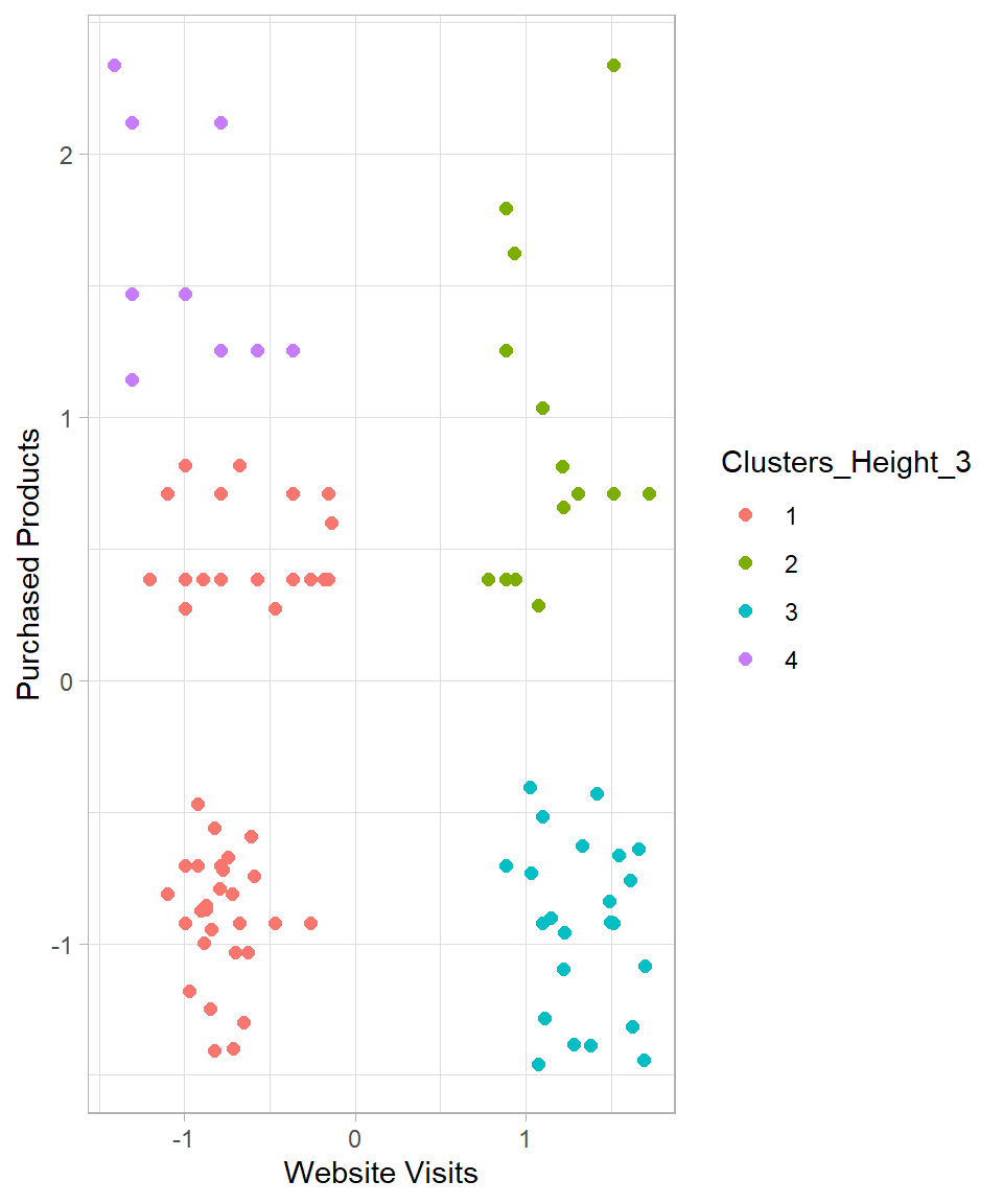
Some of the created clusters seem reasonable. However, the observations on the left side do not appear properly clustered. Setting k = 5 seems a more reasonable option. Doing so produces the following results:
# Cutting the tree to form 5 clusters
clusters_k_5 <- cutree(tree = hclust_website_visits_complete, k = 5)

# Printing clusters_k_5
clusters_k_5
[1] 1 1 1 1 2 3 4 1 5 5 1 5 1 5 4 1 1 2 2 2 2 2 1 3 5 1 5 1 4 5 1 1 2 5 1 1 1
[38] 4 5 1 5 1 4 4 4 4 4 1 2 1 2 1 2 1 1 1 5 5 2 3 5 4 4 4 4 4 4 4 4 4 4 4 4 4
[75] 4 4 4 4 4 4 4 3 3 3 3 3 3 3 3 3 3 3 3 3 3 3 3 3 3 3 3 2 2 2 2 2# Adding clusters to website_visits
website_visits <- website_visits %>%
bind_cols(Clusters_K_5 = clusters_k_5) %>%
mutate(Clusters_K_5 = as.factor(Clusters_K_5))
# Plotting website_visits with the formed clusters
website_visits %>%
ggplot(aes(x = Website_Visits,
y = Purchased_Products,
color = Clusters_K_5)) +
geom_point(size = 2) +
labs(x = "Website Visits",
y = "Purchased Products")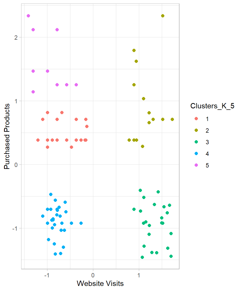
The resulting clusters seem now more reasonable. While the clusters on the right-hand side remain unchanged, the clusters on the left-hand side are now split into three different clusters instead of two.
Based on this dataset, hierarchical clustering suggests that five clusters is a suitable choice. We can describe these clusters as follows:
Cluster 1 – High Visits, High Purchases: Customers who visit the website frequently and make many purchases.
Cluster 2 – High Visits, Low Purchases: Customers who visit frequently but make few purchases.
Cluster 3 – Low Visits, Low Purchases: Customers who visit the website infrequently and make few purchases.
Cluster 4 – Low Visits, Medium Purchases: Customers who visit infrequently but make a normal/medium number of purchases.
Cluster 5 – Low Visits, High Purchases: Customers who visit infrequently but make many purchases.
Advantages and Limitations
Hierarchical clustering is a widely used method for uncovering natural groupings in data, particularly when the structure of the data is unknown. Like K-Means, it comes with both strengths and limitations that should be considered when applying it (Johnson, 1967; Everitt et al., 2011).
One of the main advantages of hierarchical clustering is its flexibility. The algorithm does not require the number of clusters to be chosen in advance; the dendrogram represents all possible clusterings, from individual observations to a single cluster containing the entire dataset. This allows analysts to explore different levels of granularity and decide later how many clusters are meaningful. Hierarchical clustering is deterministic—running the algorithm on the same data will always yield the same result, unlike K-Means, which can produce different outcomes depending on initialization. The tree-like dendrogram also provides an interpretable visual summary of how clusters are formed and related, which is especially useful in exploratory data analysis and domains like bioinformatics, marketing, and social sciences.
Another advantage is the use of different linkage methods—single, complete, average, and centroid—which define how distances between clusters are computed. This flexibility allows the method to adapt to various types of data and cluster shapes. Hierarchical clustering also does not assume clusters are spherical or evenly sized, making it more suitable than K-Means for detecting irregularly shaped or uneven clusters (Kaufman & Rousseeuw, 2009).
Despite these advantages, hierarchical clustering has notable limitations. It is computationally intensive, particularly for large datasets, because it considers all pairwise distances. Just like decision trees, hierarchical clustering is greedy and irreversible: once two clusters are merged, that decision cannot be undone, even if it turns out to be suboptimal. Early mistakes in merging can propagate through the hierarchy, potentially producing poor cluster assignments. The method is sensitive to noise and outliers, which can distort the dendrogram. Additionally, the choice of distance metric and linkage method strongly affects the resulting clusters, potentially leading to different interpretations of the same data. Finally, while dendrograms are informative, they can become cluttered and difficult to interpret for large datasets.
In summary, hierarchical clustering is a valuable tool for understanding data structure and forming interpretable clusters, particularly for small to medium-sized datasets. While K-Means excels in speed and simplicity for well-separated groups, hierarchical clustering shines when a detailed view of how clusters form and evolve across different levels of similarity is desired.
Recap
Hierarchical clustering is a versatile method for exploring the nested structure of data without pre-specifying the number of clusters. It produces a dendrogram, which shows how observations group together at different levels of similarity, helping analysts visualize and interpret cluster relationships. Hierarchical clustering is deterministic—running the algorithm on the same data always produces the same result—and can adapt to clusters of irregular shapes or uneven sizes. However, it is computationally intensive for large datasets, sensitive to noise and outliers, and irreversible: early merging decisions cannot be undone. The key is to carefully choose a linkage method, inspect the dendrogram, and determine a meaningful number of clusters to derive actionable insights from the hierarchical structure of the data.