Hypothesis Testing
Introduction
In this chapter, we will explain these fundamental ideas, starting with the standard error and moving into how we use it to test hypotheses about population parameters using the t-distribution as a way to preform hypothesis testing.
As mentioned in Chapter Introduction to Statistics, we often have a sample that we want to use to draw conclusions about the general population. If our sample is representative of that population, we would expect that the characteristics of the sample, such as the mean, are close to those of the population. However, because a sample is only a subset of the population, there is always some uncertainty in our estimates. For example, the average value in our sample is unlikely to be exactly equal to the true population mean, but we hope that it is reasonably close.
This type of uncertainty—how much a sample statistic may differ from the corresponding population parameter—is captured by the concept of the standard error. In a nutshell, the standard error measures how much a sample statistic, such as the mean, is expected to vary from the true population value due to random sampling (Urdan, 2022).
The standard error is crucial because it forms the basis for hypothesis testing, which provides a structured way to make decisions or draw conclusions about a population based on sample data. Hypothesis testing allows us to assess whether an observed effect or difference is likely to be genuine or could have occurred by chance.
In this chapter, we will explain these fundamental ideas in detail. We will begin with the concept of the standard error, showing how it quantifies sampling variability, and then move on to how it is used in hypothesis testing for population parameters, using the t-distribution to guide our conclusions.
Standard Error
Before diving into hypothesis testing, it’s essential to understand the concept of the standard error. When we calculate a statistic, such as the mean, from a sample, we expect it to differ somewhat from the population value. Assuming an unbiased sample, this difference arises due to mere random variation in the sampling process, and this random variation is called error. To keep things simple, let us focus on the standard error of the mean. As always, we assume that the population is clearly defined and the sample is a simple random sample.
The key question is: how much variation or uncertainty should we expect between the sample mean and the true population mean? This is exactly what the standard error helps us quantify.
Imagine a factory that produces boxes of ice cream, each labeled as containing 1 kilogram. In reality, due to small variations in the filling process, boxes might typically weigh anything between 950 and 1,030 grams. To monitor quality, inspectors take multiple random samples, each consisting of 10 boxes, and compute the average weight for each sample. As a result, the inspectors obtain a set of sample means—one mean per sample. These sample means form a sampling distribution of the mean, which shows how much the average weight varies from sample to sample.
This sampling distribution has its own mean and standard deviation. The mean of the sampling distribution is called the expected value of the mean, and it is approximately equal to the population mean. The standard deviation of this distribution is known as the standard error of the mean (Urdan, 2022). It tells us how much the sample mean tends to deviate, on average, from the true population mean.
Thanks to the Central Limit Theorem, this sampling distribution will approximate a normal distribution, even if the original data are not normally distributed, assuming the sample size is reasonably large. In practice though, we usually work with just one sample, not many. We calculate its average, which then becomes our best estimate of the population mean. While this sample mean is the most reasonable guess to make, we know it won’t be perfect, as it comes with some sampling error. We can estimate this uncertainty by using the sample variance, which measures the variability of individual values around the sample mean:
\[s^2 = \frac{1}{(n - 1)}\sum^n_{i = 1} (x_i - \bar{x})^2\]
Each squared difference captures how far an observation is from the sample mean. Averaging them gives us a sense of how spread out the data are. However, our interest lies not in the variation of individual values, but in the variation of sample means—that is, how much the sample mean would fluctuate if we repeated the sampling process multiple times.
It turns out that the variance of the sample mean can be approximated by:
\[Var(\bar{X}) = \frac{Var(X)}{n} = \frac{s^2}{n}\]
This formula may seem abstract at first, but it reflects an important idea: we are calculating the average of an average squared difference. Since sample variance is already an average of squared deviations, dividing by \(n\) tells us how the average of the means would vary if we took many random samples. This is the variance of the sampling distribution.
Now that we have the variance of the sample mean, we define the standard error of the mean (SEM) as its square root:
\[SE(\bar{X}) = \sqrt{\frac{s^2}{n}} = \frac{s}{\sqrt{n}}\]
The standard error tells us how much we expect the sample mean to vary due to random sampling error. In other words, while the sample mean is our best estimate of the population mean, the standard error quantifies how uncertain that estimate is. Note that:
The larger the sample size, the smaller the standard error, since increasing the denominator decreases the whole fraction.
The more spread out the data, the larger the standard error, because a larger variance indicates greater uncertainty in the estimate.
Although we’ve focused on the standard error of the mean, the same logic can be extended to other statistics, such as the median. If we could repeatedly sample from the population and compute the statistic each time, the standard deviation of that sampling distribution would give us the standard error of the statistic.
Statistical Inference and Hypothesis Testing
In real-world situations, we rarely have access to data from the entire population. Instead, we collect a sample and use it to draw conclusions about the broader population. This process is known as statistical inference, and it includes two main components:
Estimation: Using the sample to estimate unknown population characteristics, such as the average.
Hypothesis testing: Assessing specific claims about the population by comparing what we observe in the sample to what we would expect under a given assumption.
Hypothesis testing is a method that helps us decide what to believe about a population based on sample data. We start with a basic assumption, called the null hypothesis, and then ask: Does the data support this assumption, or does it suggest something different?
If the data is consistent with what we would expect under the null hypothesis, then we have no strong evidence to question it. But if the data looks unusual or far from what we would expect, we may decide that the null hypothesis is unlikely.
So, hypothesis testing helps us answer this question: Is the pattern we observe in the data substantial, or could it have happened just by chance?
The null hypothesis (denoted \(H_0\)) usually represents the status quo or no effect.
The alternative hypothesis (denoted \(H_1\) or \(H_a\)) represents a new claim or effect we want to test.
The null and alternative hypotheses are mutually exclusive and exhaustive: only one of them can be true, and together they cover all possible outcomes. This means that evidence against the null hypothesis is taken as support for the alternative.
To illustrate this concept, let’s return to the ice cream factory example. The company claims that each box contains, on average, 1000 grams of ice cream. This is a clear statement about a population parameter \(\mu\)—the average weight of all boxes produced. But what if there is doubt about whether this claim holds in practice?
To investigate, we set up two competing statements:
\(H_0: \mu = 1000\)
\(H_1: \mu \ne 1000\)
By setting up this two-sided hypothesis test, we are formally asking: is the observed sample average different enough from 1,000 grams that we should doubt the company’s claim? This approach helps us distinguish between differences that are meaningful and those that could have occurred simply by chance due to random sampling variability.
Of course, we would never expect the parameter \(\mu\) to be exactly equal to 1000. Our concern is whether \(\mu\) differs significantly from the value of 1000. More precisely, we care about whether the difference between \(\mu\) and 1000 is statistically significant. If this difference is statistically significant, then we reject the null hypothesis that \(\mu\) is equal to 1000. As a result, we turn to the alternative hypothesis, which states that \(\mu\) is not equal to 1000. This would mean that, based on our statistical inference, the average weight of a box of ice cream is significantly lower or higher than 1000 grams.
Because the focus is on the difference between the true mean and the claimed value (1000), the hypotheses can also be written as:
\(H_0: \mu - 1000 = 0\)
\(H_1: \mu - 1000 \ne 0\)
These statements are mathematically identical to the earlier formulation; the value of 1000 has simply been moved to the left-hand side of the equation.
Importantly, rejecting the null does not “prove” the alternative; it simply indicates that the data do not support the null hypothesis.
The standard error plays a central role here, as it tells us how much variation we should expect in the sample mean by chance alone. If the observed sample average is close enough to 1000 grams, we might conclude that any difference is due to normal sampling variation. But if it’s far enough away, the evidence may suggest that the true population mean is not 1000 grams, and we may question the company’s claim.
In hypothesis testing, we need to decide whether to use a two-tailed or a one-tailed approach. This depends on the type of difference we want to detect. In our example, we consider both directions because each could have serious implications:
If boxes are underfilled (less than 1000 grams), customers are not getting what they paid for. This could lead to complaints, legal consequences, and damage to the company’s reputation.
If boxes are overfilled (more than 1000 grams), the company is giving away more product than intended, which increases production costs and reduces profits.
So, a two-tailed hypothesis considers both possibilities: the true average weight could be either less than or greater than 1000 grams. In other words, it tests for any difference from the claimed value, no matter the direction. This is why our alternative hypothesis is written as \(\mu \ne 1000\). This approach is appropriate here because both underfilling and overfilling have important consequences: underfilled boxes upset customers and may lead to legal disputes, while overfilled boxes increase costs.
On the other hand, a one-tailed hypothesis focuses on just one direction of difference. For example, if the company were only concerned about boxes being underfilled, the alternative hypothesis would state \(\mu < 1000\), , and the null hypothesis would be \(\mu \geq 1000\), testing only whether the average weight is less than the claim. Alternatively, if the concern was only about overfilling, it would test whether the average is greater than 1000 grams.
Choosing between one-tailed and two-tailed hypotheses depends on what kinds of differences matter for the question at hand. In our example, since both underfilling and overfilling can have serious implications, the two-tailed approach provides a balanced way to detect any significant differences from the claim, regardless of their direction.
To judge whether the difference between the sample mean and 1000 grams is statistically significant, we need to take both the sample size and the standard deviation into account. These two factors determine the standard error, which gives us a sense of how much the sample mean would typically vary by chance alone.
Now, depending on the theoretical distribution we use, we apply different statistical tests. But the logic stays the same across all of them: we compare the observed result to what we would expect under the null hypothesis, and assess how surprising that result is based on probability.
For example, suppose we collect a sample of 25 ice cream boxes and find that the sample mean is 980 grams, with some variability. Since we don’t know the population standard deviation, we use the t-distribution (see Chapter t-Distribution) and perform a t-test for the population mean. This test helps us determine whether 980 is far enough from 1000—given the sample size and spread—to conclude that the true average weight is likely not 1000 grams.
To make this judgment, we first choose a significance level (denoted by \(\alpha\)), which represents how much risk we are willing to take of being wrong if we reject the null hypothesis. Based on this \(\alpha\), we find a critical value from the theoretical distribution (in this case, the t-distribution). The critical value acts as a cutoff point: if our test statistic goes beyond this point, the result is considered too unlikely to have happened by random chance alone. In that case, we reject the null hypothesis. For example, suppose we set our significance level at \(\alpha = 0.05\). From the t-distribution, the corresponding critical value might be about 2.1. If our calculated test statistic is \(t = 2.5\), it exceeds the critical value, meaning such a result would occur less than 5% of the time by random chance. In this case, we would reject the null hypothesis and conclude that the evidence against it is strong enough at the 5% level.
We will discuss the details of the t-test and other common statistical tests shortly. But before we go further, it’s important to remember that hypothesis testing is always based on probability. This means that mistakes are possible. There are two types of mistakes we can make:
A Type I error occurs when we reject the null hypothesis even though it is actually true. In our example, this would mean concluding that the average weight is not 1000 grams when in fact it is. We have essentially overreacted to a random fluctuation in the sample.
A Type II error happens when we fail to reject the null hypothesis even though it is false. That would mean we conclude the boxes are filled correctly when in reality they are not — we’ve missed a real problem.
Both types of errors are part of the uncertainty inherent in statistical decision-making. While we can never eliminate these risks entirely, we can control how much we are willing to tolerate, especially for Type I errors, by carefully choosing our significance level
In practice, the significance level is often set at 5% (\(\alpha = 0.05\)), meaning we accept a 5% chance of making a Type I error. However, this choice is not fixed—it depends on the context and consequences of being wrong. When the cost of an incorrect conclusion is high, such as in clinical trials for new drugs, researchers may use a smaller significance level (for example, 1% or even 0.1%) to be more cautious. In contrast, in situations where the stakes are lower, such as exploratory marketing research or small pilot studies, a higher significance level (such as 10%) may be acceptable, especially when the sample size is limited.
One Sample t-Test
Let’s return to our ice cream factory example. The company claims that each box of ice cream contains, on average, 1000 grams. To verify this claim, we take a sample of 25 boxes and measure their weights. We find that the sample mean is 1010 grams, and the sample standard deviation is 50 grams. The question we face is: does the average weight in our sample (1010 grams) differ enough from 1,000 grams to doubt the company’s claim, or could any difference simply be due to random variation?
This is the type of problem addressed by the one-sample t-test. The one-sample t-test is a statistical method used to determine whether the mean of a single sample is significantly different from a known or hypothesized population mean. It takes into account not only the difference between the sample mean and the hypothesized mean, but also the variability in the sample and the sample size, which together help us assess whether the observed difference is likely to be meaningful or could plausibly occur by chance.
So, the null and alternative hypotheses are the following:
\(H_0: \mu = 1000\)
\(H_1: \mu \ne 1000\)
Before looking at the data, we select a critical value. This value defines the threshold for how extreme our test statistic has to be in order to reject (not accept) the null hypothesis. This threshold is chosen before conducting the test, based on a pre-specified significance level, which represents the probability of making a Type I error—that is, rejecting the null hypothesis when it is actually true. To keep things simple, let us use a two-tailed test at the 5% significance level. Since we have 25 boxes, the degrees of freedom are \(n - 1 = 24\).
To conduct a t-test, we compute a t-value that tells us how far the sample mean is from the hypothesized population mean, measured in units of standard error. The formula is:
\[t = \frac{\bar{x} - \mu}{\frac{s}{\sqrt{n}}}\]
where:
\(\bar{x}\) is the sample mean
\(\mu\) is the hypothesized population mean
\(s\) is the sample standard deviation
\(n\) is the sample size
In our example, the t-value is:
\[t = \frac{1010 - 1000}{\frac{50}{\sqrt{25}}} = 1\]
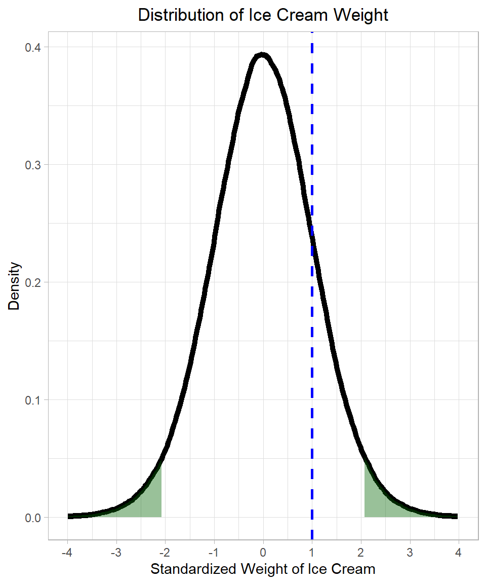
We then check where this value falls in a t-distribution with 24 degrees of freedom:
The dark green shaded areas show the rejection regions—the extreme 2.5% on each tail of the distribution. These areas are defined by the critical values from the t-distribution. At a 5% significance level, 5% of the area is split between the two tails. As we discussed in Chapter t-Distribution, we can find these critical values using the qt() function:
# 2.5% quantile of the t-distribution with 24 degrees of freedom
qt(0.025, 24)
[1] -2.063899# 97.5% quantile of the t-distribution with 24 degrees of freedom
qt(0.975, 24)[1] 2.063899In this case, the critical values are approximately -2.064 and 2.064 (remember that the t-distribution is symmetric). Since our t-value of -1 does not fall in the rejection region, we do not reject the null hypothesis. There is not enough evidence to say that the true mean differs significantly from 1000 grams.
This example illustrates the essence of hypothesis testing: we construct a theoretical (expected) distribution based on our sample statistics and then examine where the parameter value (our actual t-value in this case) falls within this distribution. If it lands in the extreme tails, we reject (do not accept) the null hypothesis. If not, we retain it.
The Concept of p-Value
The p-value helps us decide whether the result of a test is surprising, assuming the null hypothesis is true. More specifically, the p-value is the probability of observing a result at least as extreme as the one we got, if the null hypothesis is actually correct.
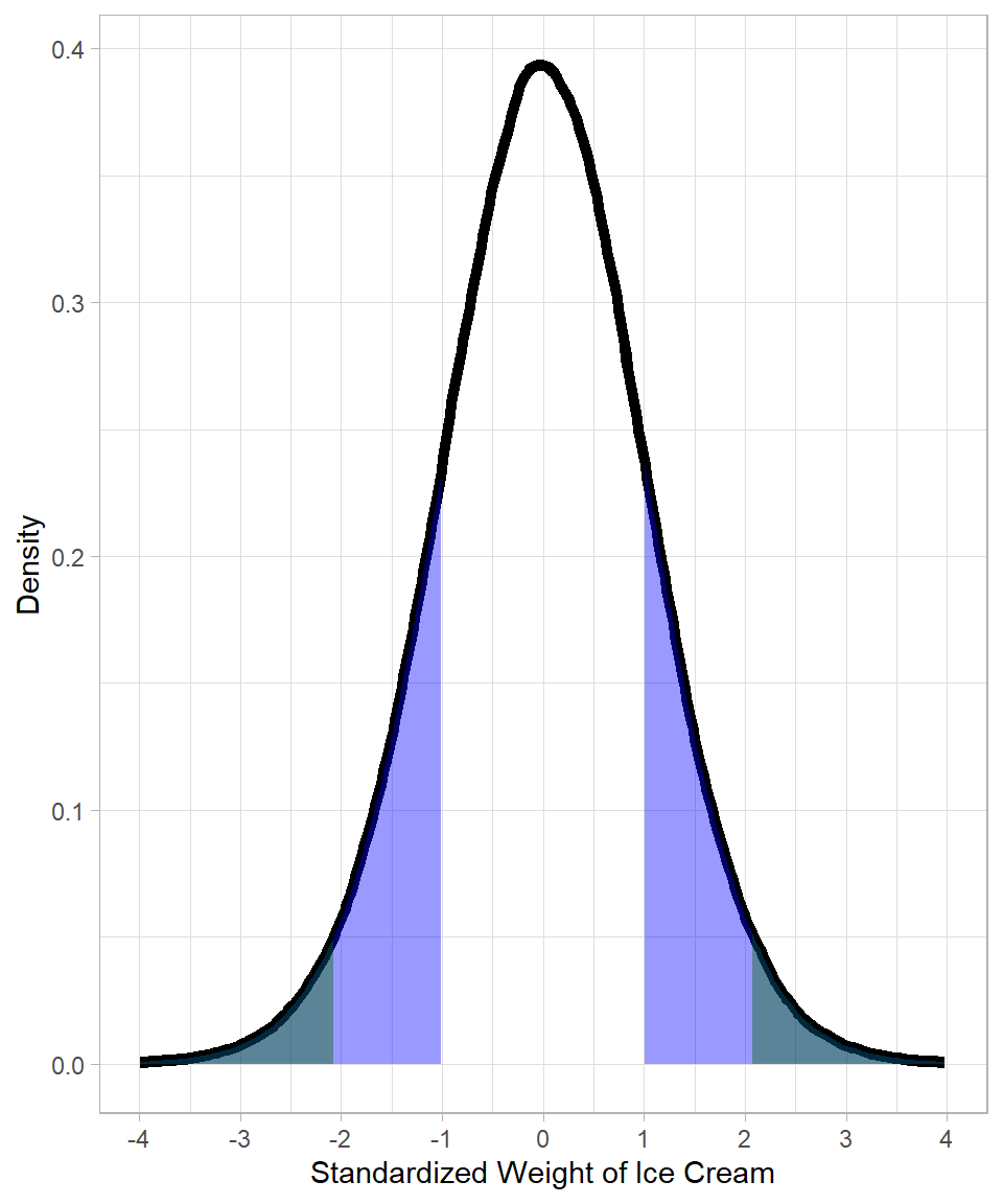
Before running the test, we already set a rejection region—these are the parts of the distribution (dark green area in Figure 20.1) we consider too far from the center to be explained by random variation (chance). The p-value is closely related to this idea: it’s the area of the distribution beyond the test statistic, on both sides in a two-tailed test.
In our example, the test statistic has a value of 1, meaning that the proportion of the distribution that would be considered at least as extreme as the one we got is the blue area below:
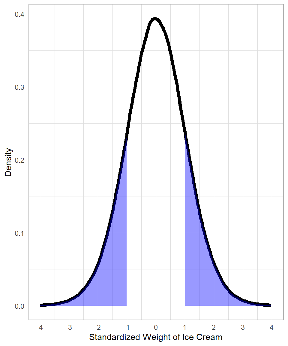
Notice how the blue area starts at point 1 of the x-axis. Because we apply a two-tailed t-test, we include the same area on the opposite side of the distribution—that is the blue are starting from -1. The blue shaded regions illustrate the p-value: the probability (proportion of the distribution) of getting a result at least as extreme as our test statistic, assuming the null hypothesis is true.
In our ice cream example, we calculated a t-value of 1. To find the p-value, we ask: how extreme is this result, assuming the true average really is 1000 grams? Since it’s a two-tailed test, we want to capture results that are just as extreme, whether above or below the mean. That’s why we look at both tails. The upper tail probability is:
# Upper tail probability
1 - pt(1, df = 24)
[1] 0.1636434To include both tails and, given the distribution is symmetric, we multiply by 2:
# Two-tailed p-value
2 * (1 - pt(1, df = 24))
[1] 0.3272869This gives us the total probability in both tails, which is the p-value.
Alternatively, we can compute each tail separately and add them:
# Two-tailed p-value (upper + lower)
(1 - pt(1, df = 24)) + pt(-1, df = 24)
[1] 0.3272869This gives the same result, just calculated manually. Either way, the p-value tells us just how likely our sample mean is, assuming nothing unusual is going on.
Notice that in this example, the conclusion is the same: we do not have enough evidence to reject the null hypothesis. The p-value is approximately 0.33 (33%), which is much larger than the significance level of 0.05 (5%).
Confidence Intervals
Hypothesis testing asks whether the data provide enough evidence to doubt a specific claim about a population parameter, such as a mean. It creates a TRUE–FALSE situation: either we have enough evidence to reject the null hypothesis, or we do not. A confidence interval, on the other hand, shows a range of plausible values for the parameter. While hypothesis testing gives a yes-or-no answer, a confidence interval shows the uncertainty around our estimate and helps us understand what values are consistent with the data (Urdan, 2022).
A confidence interval is nothing more than the edges of the area in the distribution where the values are not considered (statistically) significantly different from the mean.
Thus, a confidence interval is not a new concept—it is just a different way of expressing the same idea behind hypothesis testing. Instead of asking, “Is this value surprising enough to reject the null hypothesis?”, we ask, “What values would not be considered surprising?”
The confidence interval gives us a range around our sample estimate where we believe the true population parameter likely falls, if we were to repeat the sampling process many times. For example, a 95% confidence interval means that, in the long run, 95% of such intervals would contain the true parameter.
So, confidence intervals and hypothesis testing are two sides of the same coin:
In hypothesis testing, we compare a specific hypothesized value (such as the population mean under the null hypothesis) to determine whether it falls in the rejection region.
In confidence intervals, we calculate the boundaries of the range of plausible values and check whether the hypothesized value lies inside or outside this interval.
If the true population parameter falls outside the confidence interval, it means that the observed data are inconsistent with that value, and we would reject the corresponding null hypothesis at that confidence level.
In our ice cream example, if the 95% confidence interval for the average weight of a box does not include 1000 grams, we would reject the claim of the company at the 5% significance level. Rejecting the null hypothesis would lead us to conclude that the average box weight is most likely not 1000 grams. However, we must remember that there is still a small chance of a type I error: it could be that, by random chance, our sample happened to include unusually light (or heavy) boxes, and the sample is not fully representative of the population. If the confidence interval does include 1000 grams, we would not reject the claim.
This makes confidence intervals especially useful: not only do they tell us whether we can reject a value, but they also give us a sense of scale and uncertainty around our estimate.
To see how this concept binds with our ice cream example, let’s try to calculate the confidence interval.
The general formula for a confidence interval around a mean for a t-distribution is:
\[CI_{*} = \bar{x} \pm t_{*} \times SE\]
Where:
\(CI_{*}\) is the confidence interval based on some significance level. For instance, the 95% confidence interval is \(CI_{95}\).
\(\bar{x}\) is the sample mean
\(t_*\) is the critical value from the t-distribution based on the chosen confidence level and degrees of freedom. For example, with a 5% significance level, the critical value \(t_{95}\) marks the cutoff where we accept 95% of the distribution and reject the extreme 5%.
\(SE = \frac{s}{\sqrt{n}}\) is the standard error of the mean
\(s\) is the sample standard deviation
\(n\) is the sample size
In our ice cream example:
\(\bar{x} = 1010\)
\(s = 50\)
\(n = 25\), so the degrees of freedom is \(n - 1 = 24\)
For a 95% confidence interval with 24 degrees of freedom, the critical t-value is approximately \(t_{95} = 2.064\)
The standard error is \(SE = \frac{50}{\sqrt{25}} = 10\)
Plugging into the formula:
\[CI_{95} = 1010 \pm 2.064 \times 10 = 1010 \pm 20.64\]
So, the 95% confidence interval is:
\[(989.36, 1030.64)\]
This tells us that if we were to repeat the sampling process many times, about 95% of the resulting confidence intervals would contain the true population mean. In our particular sample, the confidence interval provides a range of plausible values for the true mean. Since the interval includes values close to 1000 grams, we do not have enough evidence to reject the company’s claim. In other words, the sample is consistent with the hypothesized mean of 1000 grams.
Practical Significance
Before we wrap up this chapter, it is important to emphasize the difference between statistical significance and practical significance. Statistical significance tells us whether a result is likely due to chance. Essentially, it measures how far a parameter value is from a sample value in terms of standard error units.
On the other hand, practical significance considers whether the difference is large enough to be important or noticeable in real life. It is often more subjective and depends on the context and the perspective of the person evaluating the results.
For example, if the ice cream factory’s average box weight is found to be 995 grams instead of the claimed 1000 grams, an inspector might see this as a serious issue because even a small underfill can affect product quality and regulatory compliance. However, a customer buying the ice cream might not even notice this slight difference, and it would likely not affect their satisfaction. This shows that a result can be statistically significant but not necessarily practically meaningful for everyone.
Recap
In this chapter, we explored the concept of standard error, which quantifies the uncertainty in a sample statistic, especially the sample mean. Because sample means vary due to random sampling, the standard error tells us how much the sample mean is expected to fluctuate around the true population mean. This helps us understand the precision of our estimates.
The chapter also introduced statistical inference, including estimation and hypothesis testing, which are tools for drawing conclusions about populations from sample data.
We focused on the example of an ice cream factory’s box weights to illustrate hypothesis testing. We defined the null hypothesis (no difference from the claimed weight) and the alternative hypothesis (a difference exists), and discussed the importance of choosing between a two-tailed or one-tailed test based on the research question.
Finally, we introduced the one sample t-test, which compares a sample mean to a hypothesized population mean when the population standard deviation is unknown. We calculated the test statistic using the sample mean, sample standard deviation, and sample size, and showed how to interpret it in the context of the t-distribution to make a decision about the null hypothesis.
Throughout, we highlighted the role of probability and the possibility of errors—rejecting a true null hypothesis (Type I error) or failing to reject a false one (Type II error)—emphasizing that statistical decisions are always about managing uncertainty rather than providing absolute truths.