# Importing Customer_Churn
customer_churn <- read.csv("C:/Users/User/Desktop/Data Sets/Customer_Churn.csv")

# Printing the first 6 rows
head(customer_churn)Importing Data
Introduction
In this chapter, we discuss the main topics regarding data imports. Understanding how to effectively import data is a crucial skill for data analysis, as it forms the foundation upon which all subsequent analysis is built. As such, the principles we will cover are broadly applicable across various software environments.
Spreadsheets and File Types
Data sets are typically stored in all kinds of formats. Probably the most common type is the table form or electronic spreadsheet (e.g., Excel format). A spreadsheet is similar to a data frame or matrix, because it consists of rows and columns. The type of file determines how we import it into R. Common file types include Excel workbooks, CSV files, or text files with specific delimiters such as tabs or semicolons. For instance, a CSV file (Comma-Separated Values) uses commas to separate values within each row. Understanding these file types is crucial because it influences how data is read into R using appropriate functions or packages. For instance, the file Customer_Churn below is seen with a text editor:
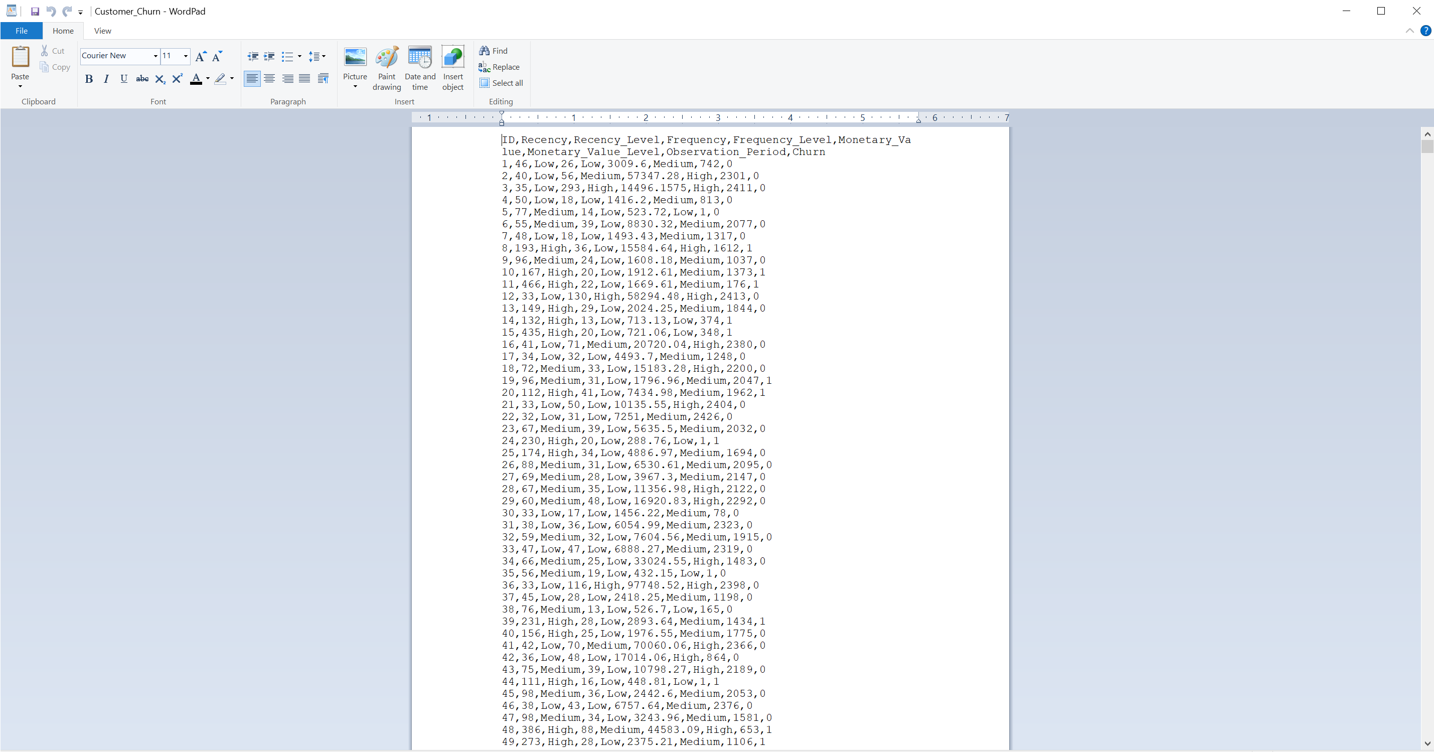
The first row contains headers, which might appear wrapped due to length but, in terms of structure, they are still a single row. By understanding the file type and structure, we can accurately import our data in R.
Paths and the Working Directory
Except for the file type, we need to know the path of a file. The path of a file essentially denotes where the file is stored. Usually, we can have these files in organized folders, which are called directories. Although the names may not be so intuitive, the important thing to remember is that, to import a file in RStudio, we need to know its type and where it is. To understand the terminology, suppose we have a csv file called Customer_Churn in a folder called Data Sets. A possible path in that case would be C:/Users/User/Desktop/Data Set/Customer_Churn.csv. Let’s break it down:
Full path:
C:/Users/User/Desktop/Data Sets/Customer_Churn.csvDirectory Path:
C:/Users/User/Desktop/Data SetsDirectory:
Data SetsFile:
Customer_Churn.csv
So, by using the full path, we can import a data set in R. To see how this works in practice, we implement what we just described. The built-in function to import a csv file in R is the function read.csv(). Inside the function we specify the full path and we can store the data in an object directly. In our example, we give the name customer_churn to the object in which we want to store the imported data:
  ID Recency Recency_Level Frequency Frequency_Level Monetary_Value
1  1      46           Low        26             Low        3009.60
2  2      40           Low        56          Medium       57347.28
3  3      35           Low       293            High       14496.16
4  4      50           Low        18             Low        1416.20
5  5      77        Medium        14             Low         523.72
6  6      55        Medium        39             Low        8830.32
  Monetary_Value_Level Observation_Period Churn
1               Medium                742     0
2                 High               2301     0
3                 High               2411     0
4               Medium                813     0
5                  Low                  1     0
6               Medium               2077     0
When we work with R though, we are always located “somewhere” in the computer in which we work. In other words, R assumes that we have a specific path, from which we work. This is called our working directory. With working directory, there is no need to specify the full path every time when we import a data set; we can simply use the file name instead of the full path inside the function. Before we see how this works, let’s check our current working directory. For this, we can use the function getwd():
# Getting working directory
getwd()
[1] "C:/Users/User/Document"We see that our working directory is C:/Users/User/Document (your directory will probably be different). To change the working directory, we can use the function setwd(). For instance, suppose we want to change the working directory from C:/Users/User/Document to C:/Users/User/Desktop/Data Sets. To do this, we enter the desired directory path inside the parenthesis:
# Changing working directory
setwd("C:/Users/User/Desktop/Data Sets")
Now, if we use the getwd() again, we see that our working directory is different:
# Getting working directory
getwd()
[1] "C:/Users/User/Desktop/Data Sets"As our working directory is the Data Sets directory, we can now use the read.csv() function by only filling the name of the file in the parenthesis:
# Importing Customer_Churn
customer_churn <- read.csv("Customer_Churn.csv")

# Printing the first 6 rows
head(customer_churn)
ID Recency Recency_Level Frequency Frequency_Level Monetary_Value
1 1 46 Low 26 Low 3009.60
2 2 40 Low 56 Medium 57347.28
3 3 35 Low 293 High 14496.16
4 4 50 Low 18 Low 1416.20
5 5 77 Medium 14 Low 523.72
6 6 55 Medium 39 Low 8830.32
Monetary_Value_Level Observation_Period Churn
1 Medium 742 0
2 High 2301 0
3 High 2411 0
4 Medium 813 0
5 Low 1 0
6 Medium 2077 0We see that the data import occurs successfully. In this way, we can import different data sets quite efficiently. Another advantage is that, when we share our R script, our code is more readable and other people can easily run the script under the assumption that their working directory contains the same data set. Note that when a file is located in the working directory, we can still use the full path if we want; the result would be exactly the same.
Importing Data in RStudio
Now that we understand the concepts of path and directory, we can examine in practice how to import a data set in R by using the RStudio functionality. To keep things simple, we import the same data set with the same full path as described. So, the csv file that we import is called Customer_Churn and the directory path is C:/Users/User/Desktop/Data Sets. As shown earlier, we can use the read.csv() function to import this data set.
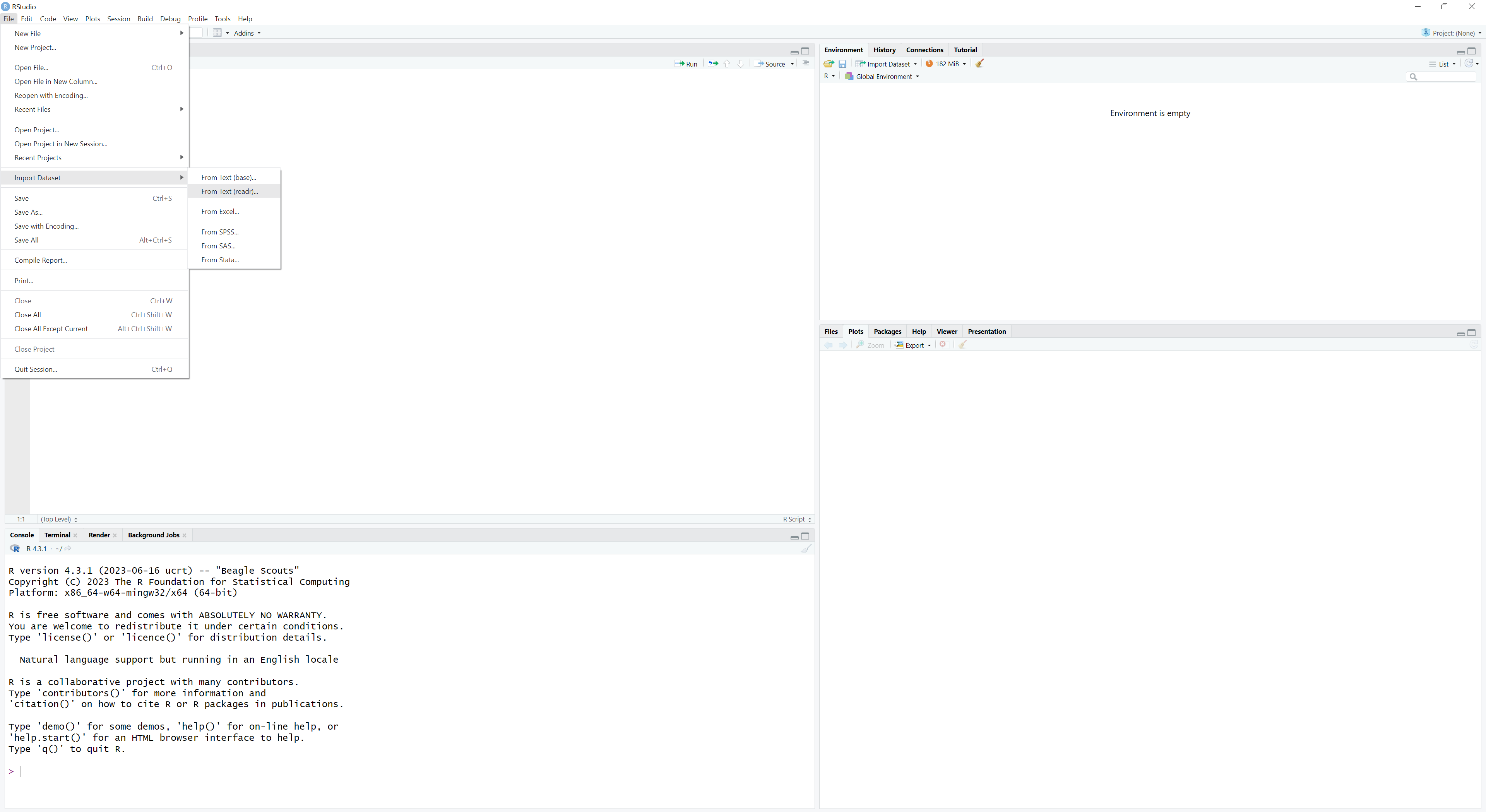
However, RStudio also provides a user-friendly functionality that can help us import our data sets in a relatively straightforward manner. By choosing File -> Import Dataset, we can see that RStudio provides us with different options, such as From Text (readr)…. By clicking this option, we will see the following output:
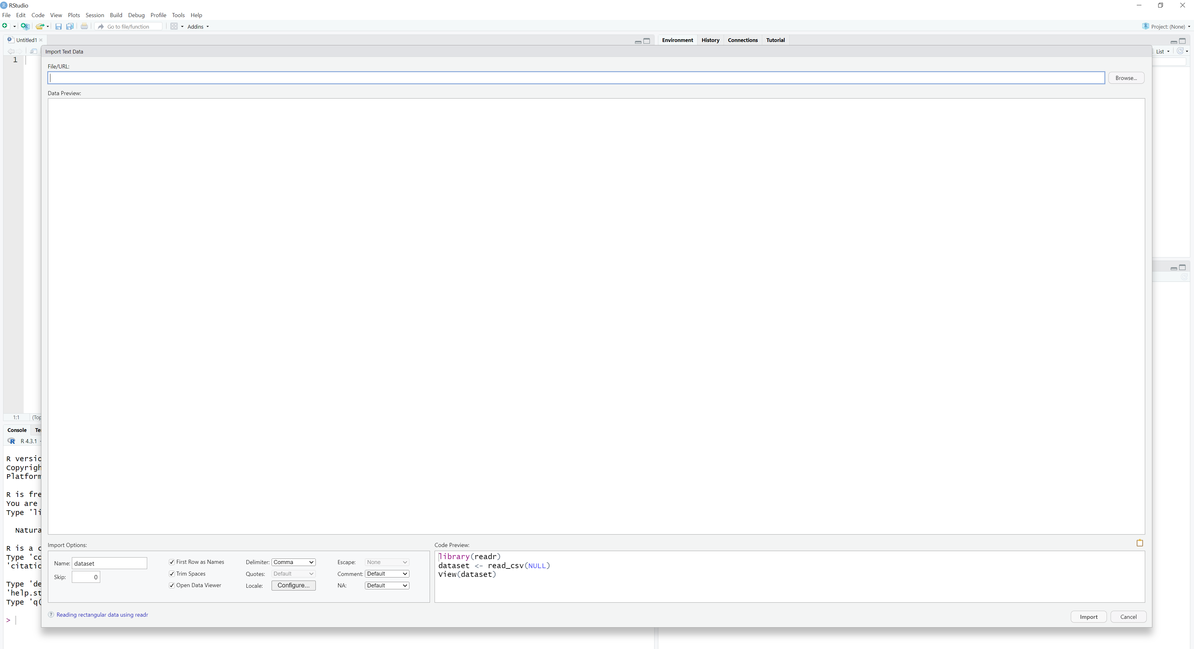
To find the file in our computer, we click the option Browse on the top right corner and find the file by browsing in our computer system. When we find the file we want, we click on it and visualize it on the emerging table:
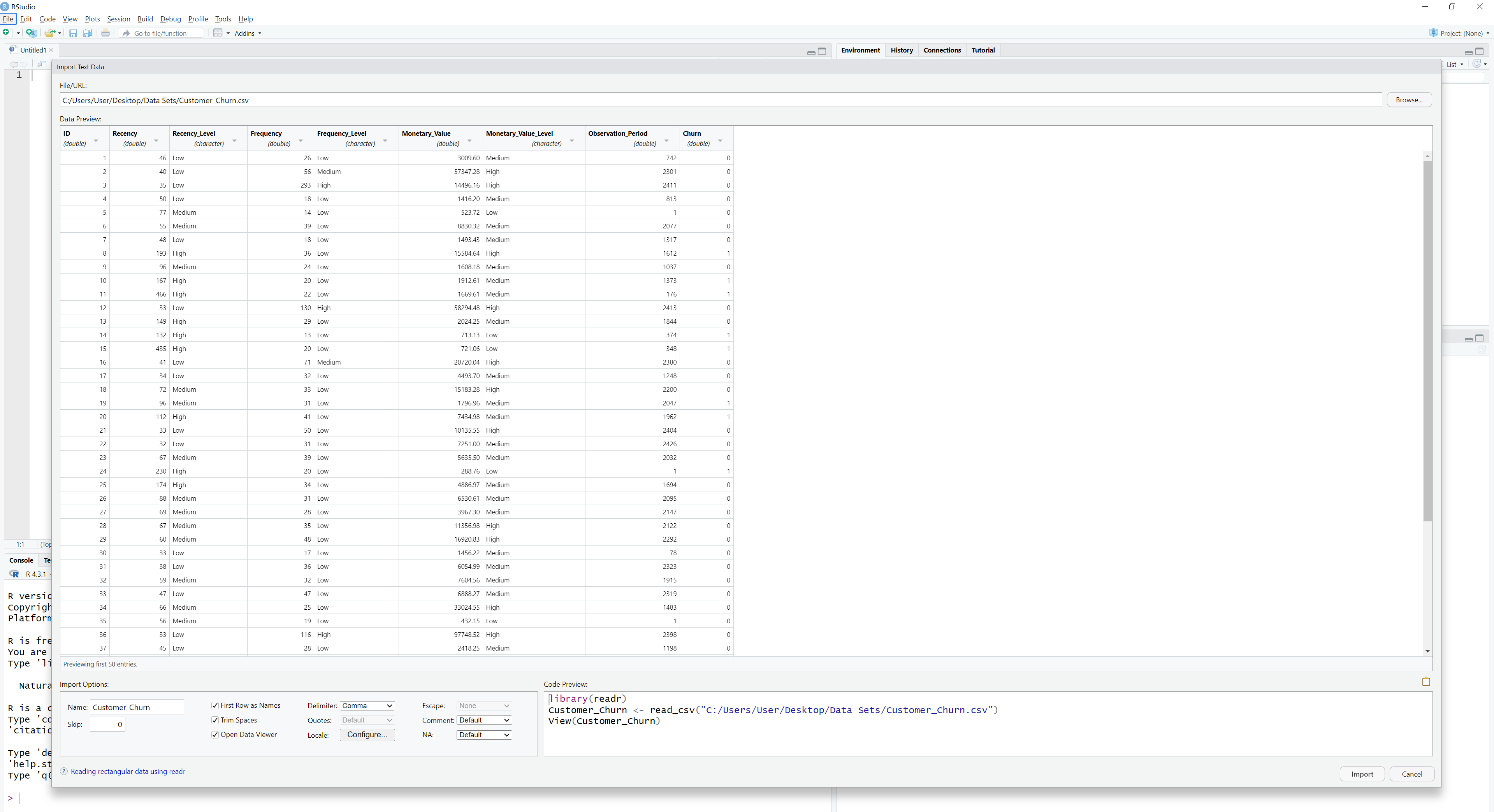
Here, we have a number of options that allow us to change how RStudio imports the file. In this way, we see exactly what RStudio will import and, respectively, we can make adjustments before the import takes place. Lastly, we see the exact R code that makes the import on the bottom right corner on the bottom right corner. This is very valuable because not only can we use this code later, but also we can learn how to import a data set by coding directly on the console. In this example, we note that RStudio used the readr package and the function read_csv() to make this import possible. This function can be thought of as an advanced version of the read.csv() function. The details are not important at this point; our goal is to capture the intuition about paths, directory and the overall functionality of RStudio regarding data import.
Importing Data from GitHub
In addition to importing files from local directories, R also allows direct data import from online sources such as GitHub repositories. GitHub is a web-based platform for hosting and sharing code, datasets, and collaborative projects. It is one of the most widely used platforms for collaboration and storing code. Although GitHub offers many features, we don’t need to explore them in detail here. Our goal is simply to see how we can import a dataset from such platforms. Many of these datasets can be accessed directly via their URLs. For instance, suppose we want to import the publicly available customer_churn dataset from GitHub: https://github.com/DataKortex/Data-Sets/blob/main/customer_churn.csv
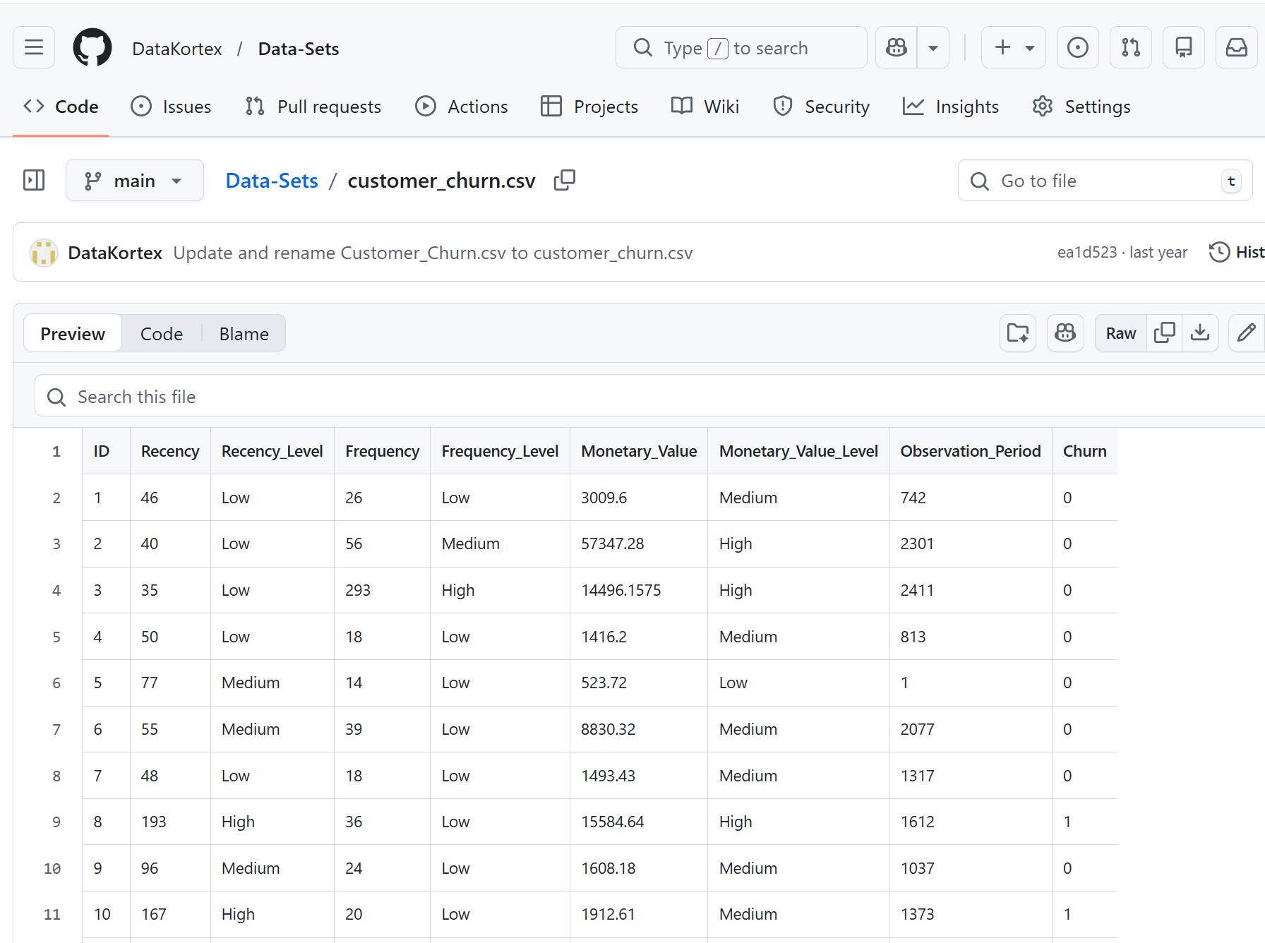
By clicking the Raw tab on GitHub, we access the raw CSV file that can be directly imported into R:
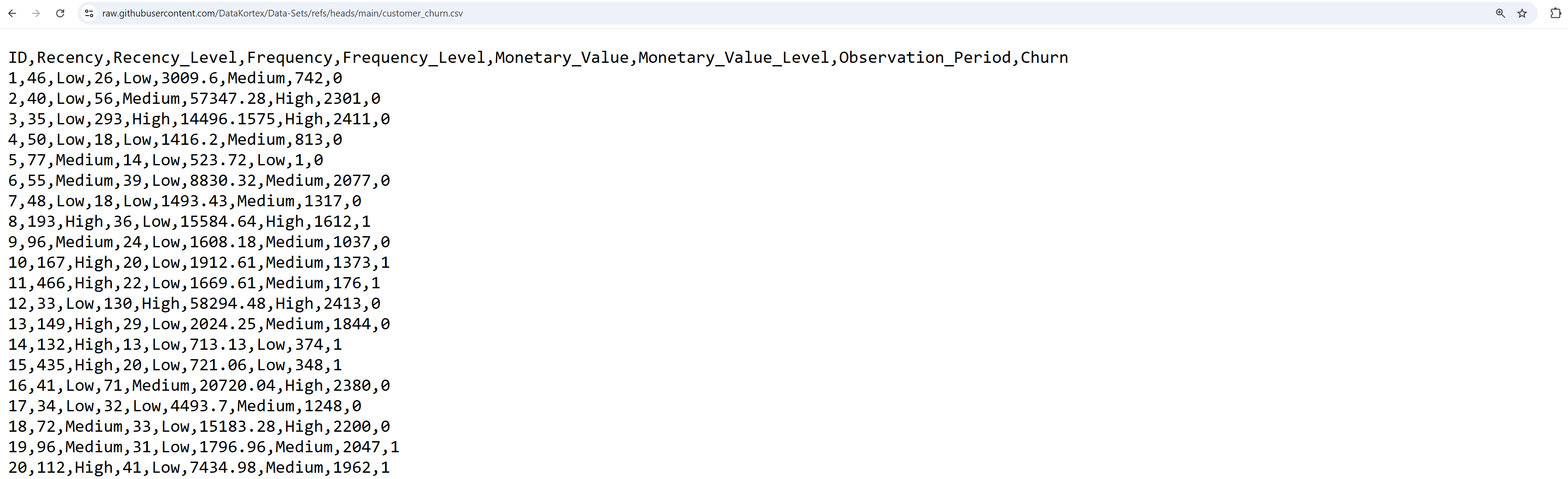
The format is still CSV (values separated by commas), which allows us to import the dataset using either read.csv() or read_csv() by providing the raw file URL:
# Importing customer_churn from GitHub
customer_churn <- read.csv("https://raw.githubusercontent.com/DataKortex/Data-Sets/refs/heads/main/customer_churn.csv")

# Printing the first 6 rows
head(customer_churn)
ID Recency Recency_Level Frequency Frequency_Level Monetary_Value
1 1 46 Low 26 Low 3009.60
2 2 40 Low 56 Medium 57347.28
3 3 35 Low 293 High 14496.16
4 4 50 Low 18 Low 1416.20
5 5 77 Medium 14 Low 523.72
6 6 55 Medium 39 Low 8830.32
Monetary_Value_Level Observation_Period Churn
1 Medium 742 0
2 High 2301 0
3 High 2411 0
4 Medium 813 0
5 Low 1 0
6 Medium 2077 0Notice that the local file path does not matter in this case, as we are importing the dataset directly from the web.
This functionality is particularly useful for reproducible research and collaborative projects. It allows all users to access the same dataset from a shared online location without manually downloading files. As long as the URL remains valid, the dataset can be imported consistently across different systems and environments.
Importing Data from Other Sources
It is possible to import data in R from various sources, including relational database platforms such as MySQL, as well as directly from web pages via URLs (just like we did earlier). Additionally, R can be used for web scraping, which involves extracting data from HTML or directly from web pages. Given the variety of data sources, it’s impractical to cover every possible method in detail in this introductory chapter. However, the core idea remains the same: we need to guide R to the location of the data and specify the appropriate function for importing it, as different file types require different functions.