In this chapter, we explore advanced topics in linear regression that extend beyond modeling a response variable with basic predictors. We demonstrate how to apply transformations, such as logarithms and squared terms, and examine their impact on interpretation and inference. We also introduce dummy variables to capture group differences, and show how interaction terms allow for group-specific effects.
The focus is not only on building more flexible models, but also on interpreting them, especially as complexity increases with transformations and interactions. Emphasis is placed on developing an intuitive grasp of these extensions and their practical meaning. The chapter concludes with a comprehensive regression model that brings together many of these techniques in a unified example.
The Simplest Form of Regression
In Chapter Simple Linear Regression, we examined the bivariate case, where the dependent variable is regressed on a single independent variable. While this is often considered the simplest form of regression, the truly simplest regression model includes only an intercept—that is, no independent variables at all.
Let us set up the environment and use the lm() function in R to regress the variable Revenue from the eshop_revenues dataset on a constant term alone. To specify a regression model with only an intercept, we include the number 1 after the tilde (~):
# Librarieslibrary(tidyverse)# Setting optionsoptions(scipen =999, digits =3)# Importing eshop_revenueseshop_revenues <-read_csv("https://raw.githubusercontent.com/DataKortex/Data-Sets/refs/heads/main/eshop_revenues.csv")# Fitting a linear regression modellm_model <-lm(Revenue ~1, data = eshop_revenues)# Printing coefficientssummary(lm_model)
Call:
lm(formula = Revenue ~ 1, data = eshop_revenues)

Residuals:
   Min     1Q Median     3Q    Max
-15734 -11475  -5294   6267  76867

Coefficients:
            Estimate Std. Error t value            Pr(>|t|)
(Intercept)    16102       1414    11.4 <0.0000000000000002 ***
---
Signif. codes:  0 '***' 0.001 '**' 0.01 '*' 0.05 '.' 0.1 ' ' 1

Residual standard error: 16100 on 129 degrees of freedom
The summary() function outputs the estimated intercept coefficient only. This estimated intercept corresponds exactly to the mean of the dependent variable Revenue. Furthermore, the standard error reported for the intercept is equivalent to the standard error of the mean of Revenue. We can verify this by calculating these values directly:
# Calculating the meanmean(eshop_revenues$Revenue)
[1] 16102
# Calculating the standard errorsd(eshop_revenues$Revenue) /sqrt(nrow(eshop_revenues))
[1] 1414
These calculations yield the same values as the regression output.
The t-value and p-value provided in the regression summary correspond to those from a one-sample t-test comparing the mean of Revenue to zero. In other words, this regression with only an intercept tests whether the mean of the dependent variable differs significantly from zero.
Because this model contains no explanatory variables, it does not explain any variance in the dependent variable. Consequently, the coefficient of determination \(R^2\) is exactly zero. Additionally, no F-statistic is provided because the model includes only an intercept term, meaning there are no predictors to jointly test for significance.
This simplest regression model essentially serves as a baseline or null model. It represents the expected value of the dependent variable when no other information is used for prediction. More complex models with predictors can be compared against this baseline to evaluate their explanatory power
Regression through the Origin
Just like we can remove the independent variable from a simple linear regression model, we can also remove the intercept and keep only the independent variable. Recall that the intercept represents the expected value of the dependent variable when the independent variable equals zero. In this case, however, by removing the intercept, we force the regression line to pass through the origin, meaning that when \(x = 0\), the predicted value of the dependent variable is also zero.
As a result, the slope coefficient will adjust to compensate for the missing intercept. This change can substantially alter the estimated relationship between the variables, often increasing or decreasing the slope depending on the data distribution.
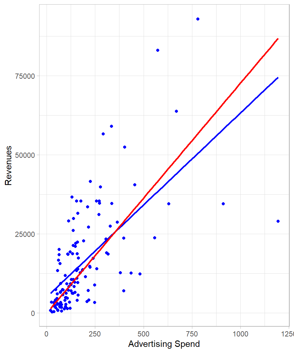
The plot below shows the regression lines of Revenue on Ad_Spend, with the standard regression line including an intercept in blue, and the regression through the origin shown in red:
Figure 26.1: Comparing linear regression lines with and without intercepts.
It is clear from the plot that the slope—the steepness of the line—changes when we force the regression line to pass through the origin at \((0, 0)\).
To run a regression through the origin in R, we simply include 0 after the tilde in the model formula:
# Fitting a linear regression modellm_model <-lm(Revenue ~0+ Ad_Spend, data = eshop_revenues)# Printing coefficientssummary(lm_model)
Call:
lm(formula = Revenue ~ 0 + Ad_Spend, data = eshop_revenues)

Residuals:
   Min     1Q Median     3Q    Max
-57774  -3136    165   9979  41437

Coefficients:
         Estimate Std. Error t value            Pr(>|t|)
Ad_Spend     72.7        4.4    16.5 <0.0000000000000002 ***
---
Signif. codes:  0 '***' 0.001 '**' 0.01 '*' 0.05 '.' 0.1 ' ' 1

Residual standard error: 12900 on 129 degrees of freedom
Multiple R-squared:  0.679, Adjusted R-squared:  0.676
F-statistic:  273 on 1 and 129 DF,  p-value: <0.0000000000000002
Although this approach may be reasonable in some contexts, such as when the dependent variable cannot logically take negative values and a negative intercept would be nonsensical, we must exercise caution. Omitting the intercept generally results in biased coefficient estimates because the model is constrained to fit through the origin regardless of the true relationship in the data (Wooldridge, 2022).
Furthermore, the coefficient of determination \(R^2\) can be misleadingly high in regressions through the origin. This occurs because the usual definition of \(R^2\) assumes a model with an intercept, and removing it changes the total sum of squares calculation. Consequently, the adjusted \(R^2\) is also affected and cannot be interpreted in the same way as in models with an intercept.
Mathematically, the traditional \(R^2\) is computed as:
\[R^2 = 1 - \frac{\text{RSS}}{\text{TSS}}\]
where \(\text{RSS}\) is the residual sum of squares, and \(\text{TSS}\) is the total sum of squares calculated relative to the mean of the dependent variable. However, in regression through the origin, since the intercept is zero, the \(\text{TSS}\) is calculated relative to zero rather than the mean, generally inflating the \(R^2\) value. Therefore, \(R^2\) in this case does not represent the proportion of variance explained in the same way and should be interpreted with care. Actually, regression through the origin can produce even a negative \(R^2\). Because of this, when \(R^2\) is an important metric and regression through the origin is necessary, alternative definitions or adjusted versions of \(R^2\) are often used to better reflect model fit.
Regression with a Dummy Variable
Up to this point, we have seen how linear regression can be applied when the independent variables are continuous. However, it is also possible—and quite common in practice—to include categorical variables in a linear regression model. The simplest case is when a categorical variable has only two levels, which we can represent using a dummy (binary) variable. The interpretation of coefficients in this case differs slightly from that of continuous predictors.
When we include a dummy variable in a regression model, the equation can be written as:
\[y = \beta_0 + \gamma_1 x_1\]
where \(x_1\) is a dummy variable that takes the value 1 for one group and 0 for the other. The intercept \(\beta_0\) represents the mean of the reference group (where \(x_1 = 0\)), and the coefficient \(\gamma_1\) captures the mean difference between the two groups. This means that the predicted value of \(y\) for the group coded as 1 is \(\beta_0 + \gamma_1\), while for the group coded as 0 it is simply \(\beta_0\). In essence, regression with a dummy variable estimates the group means and compares them directly.
The Dummy Variable Trap and Reference Groups
We could create a separate dummy variable for each group. In this case, our model would be:
\[y = \beta_0 +\gamma_1 x_1 + \gamma_2 x_2\]
where \(x_1\) takes the value 1 for the first group and 0 otherwise, and \(x_2\) takes the value 1 for the second group and 0 otherwise. At first glance, this seems like a natural way to include all groups explicitly in the model. However, this approach leads to perfect collinearity, a situation where one variable can be perfectly predicted from the others. In this case, the sum of the dummy variables \(x_1 + x_2\) always equals 1, which is the same as a column of ones—exactly what the intercept \(\beta_0\) captures. As a result, the model cannot uniquely estimate all parameters. This issue is known as the dummy variable trap. To avoid it, we always exclude one of the dummy variables—typically the reference group—so that its effect is absorbed by the intercept.
In our dataset, the variable New_Product is such a dummy variable, indicating whether the product is new or not. Although it appears numeric in R (as it takes values 0 or 1), it is conceptually a categorical variable.
# Fitting a linear regression modellm_model <-lm(Revenue ~ New_Product, data = eshop_revenues)# Printing coefficientssummary(lm_model)
Call:
lm(formula = Revenue ~ New_Product, data = eshop_revenues)

Residuals:
   Min     1Q Median     3Q    Max
-19259 -11291  -4211   4162  72009

Coefficients:
            Estimate Std. Error t value            Pr(>|t|)
(Intercept)    14768       1583    9.33 0.00000000000000041 ***
New_Product     6192       3410    1.82               0.072 .
---
Signif. codes:  0 '***' 0.001 '**' 0.01 '*' 0.05 '.' 0.1 ' ' 1

Residual standard error: 16000 on 128 degrees of freedom
Multiple R-squared:  0.0251,    Adjusted R-squared:  0.0175
F-statistic:  3.3 on 1 and 128 DF,  p-value: 0.0718
The estimated coefficient of New_Product is 6,192 and is statistically significant at the 10% significance level. This means that, on average, new products are associated with an increase of approximately 6,192 in revenue, compared to non-new products. The intercept is 14,768, which represents the expected revenue when New_Product = 0—that is, when the product is not new.
A regression model with a single dummy variable is equivalent to performing a two-sample independent t-test, under the assumption of equal variances across the two groups. In the context of linear regression, the assumption of equal variances corresponds to the homoskedasticity assumption. Therefore, the t-value and p-value reported for the dummy variable’s coefficient match those that would be obtained from a traditional two-sample t-test. We can actually confirm this by using the t.test() function:
# Performing a t-testt.test(Revenue ~ New_Product, data = eshop_revenues, var.equal =TRUE)
    Two Sample t-test

data:  Revenue by New_Product
t = -2, df = 128, p-value = 0.07
alternative hypothesis: true difference in means between group 0 and group 1 is not equal to 0
95 percent confidence interval:
 -12939    556
sample estimates:
mean in group 0 mean in group 1
          14768           20960
We also see that we can apply the t.test() function in a similar fashion as we do with the lm() function. The other option would be to have the revenues in the form of two separate vectors—one for the new products and one for the non-new products—and apply the t.test() as we explained in Chapter Statistical Tests.
Regression with Many Dummy Variables
Instead of two groups, we may have three or more groups defined by a categorical variable. For example, suppose we want to classify our products into pricing categories: low, medium, and high. For simplicity, we create a new variable called Price_Level that takes on four values based on the product’s price:
1 if the price is below 50
2 if the price is above or equal to 50 and below 100
3 if the price is above or equal to 100 and below 150
4 if the price is above 150
We can create this variable using the case_when() function from the dplyr package:
Once we have this variable, we have two main options for including it in a linear regression model. The first option is to this variable as a continuous variable and use the lm() function as usual:
# Fitting a linear regression model with Price_Level as one variablelm(Revenue ~ Price_Level, data = eshop_revenues) %>%summary()
Call:
lm(formula = Revenue ~ Price_Level, data = eshop_revenues)

Residuals:
   Min     1Q Median     3Q    Max
-18957  -9522  -4728   8065  75406

Coefficients:
            Estimate Std. Error t value        Pr(>|t|)
(Intercept)    25163       3241    7.76 0.0000000000023 ***
Price_Level    -3800       1232   -3.08          0.0025 **
---
Signif. codes:  0 '***' 0.001 '**' 0.01 '*' 0.05 '.' 0.1 ' ' 1

Residual standard error: 15600 on 128 degrees of freedom
Multiple R-squared:  0.0692,    Adjusted R-squared:  0.0619
F-statistic: 9.52 on 1 and 128 DF,  p-value: 0.00249
The estimated coefficient for Price_Level is -3,800 and statistically significant at the 1% significance level. This suggests that, on average, moving from one price level to the next (e.g., from Level 1 to Level 2) is associated with a decrease in revenue of about 3,800 units. However, this interpretation assumes that the levels are equally spaced and that the relationship between price levels and revenue is linear. This may not be a valid assumption, especially if the effect of price on revenue is non-linear or varies irregularly across levels.
A more flexible approach is to treat Price_Level as a factor. This tells R to treat each level as a distinct category and to include dummy variables (one for each level except the reference category) in the model. To do this, we can either transform the variable Price_Level into a factor before we apply the lm() function or use the factor() function directly within the lm() function. The following code shows the second option.
# Fitting a linear regression model with Price_Level as dummy variableslm(Revenue ~factor(Price_Level), data = eshop_revenues) %>%summary()
Call:
lm(formula = Revenue ~ factor(Price_Level), data = eshop_revenues)

Residuals:
   Min     1Q Median     3Q    Max
-19109  -9703  -4379   7343  71713

Coefficients:
                     Estimate Std. Error t value      Pr(>|t|)
(Intercept)             18103       2693    6.72 0.00000000056 ***
factor(Price_Level)2     3153       3530    0.89         0.373
factor(Price_Level)3    -5232       4456   -1.17         0.242
factor(Price_Level)4    -9555       3839   -2.49         0.014 *
---
Signif. codes:  0 '***' 0.001 '**' 0.01 '*' 0.05 '.' 0.1 ' ' 1

Residual standard error: 15500 on 126 degrees of freedom
Multiple R-squared:  0.101, Adjusted R-squared:  0.0793
F-statistic:  4.7 on 3 and 126 DF,  p-value: 0.00379
This approach of using dummy variables allows each level of Price_Level to have its own estimated effect on revenue. R will automatically drop the first level (in this case, Level 1) and treat it as the reference group. The reported coefficients then indicate how much higher or lower the revenue is for each price level compared to the reference group.
Removing the Intercept for Multiple Groups
When we have a categorical variable, we can actually remove the intercept in order to change the interpretation of the coefficients. For example, removing the intercept in the previous example gives:
# Fitting a linear regression model with Price_Level as dummy variableslm(Revenue ~0+factor(Price_Level), data = eshop_revenues) %>%summary()
Call:
lm(formula = Revenue ~ 0 + factor(Price_Level), data = eshop_revenues)

Residuals:
   Min     1Q Median     3Q    Max
-19109  -9703  -4379   7343  71713

Coefficients:
                     Estimate Std. Error t value           Pr(>|t|)
factor(Price_Level)1    18103       2693    6.72 0.0000000005596277 ***
factor(Price_Level)2    21256       2281    9.32 0.0000000000000005 ***
factor(Price_Level)3    12870       3550    3.63            0.00042 ***
factor(Price_Level)4     8547       2735    3.12            0.00221 **
---
Signif. codes:  0 '***' 0.001 '**' 0.01 '*' 0.05 '.' 0.1 ' ' 1

Residual standard error: 15500 on 126 degrees of freedom
Multiple R-squared:  0.551, Adjusted R-squared:  0.537
F-statistic: 38.7 on 4 and 126 DF,  p-value: <0.0000000000000002
The estimated coefficients now represent the average value for each group. These coefficients remain unbiased because we are not “forcing” any single intercept to be zero; instead, each group effectively gets its own intercept.
Note that \(R^2\) and adjusted \(R^2\) may differ from the model with a single intercept because the reference point for the mean is now the group-specific means rather than the overall mean. As a result, the proportion of variance explained is calculated relative to these group-specific averages, which can change the interpretation of model fit.
In practice, the factor approach is often preferred when the numeric levels represent distinct categories with no natural ordering or when the effect of moving from one level to another is not expected to be linear or uniform.
ANOVA as a Special Case of Linear Regression
A linear regression model with dummy variables is mathematically equivalent to the F-test ANOVA we discussed in chapter Statistical Tests. In fact, if we use the aov() or anova() functions in R on the same model, you will obtain the exact same F-statistic and reach the same conclusions about group differences. This reinforces the idea that ANOVA is simply a special case of linear regression, where the predictors are dummy variables representing each group.
Beta Coefficients
In Chapter Simple Linear Regression, we discussed how the units of measurement affect the interpretation of coefficients—changing the scale of a variable alters the size of the coefficient, though not its underlying relationship with the dependent variable. However, in many situations, we are not interested in the original units of the variables at all. Instead, we are interested in comparing the relative strength of the relationships between variables, which requires a common scale (Wooldridge, 2022).
To achieve this, we can standardize our variables before applying linear regression. Standardization transforms each variable to have a mean of 0 and a standard deviation of 1. When we perform regression on standardized variables, the resulting coefficients are called beta coefficients or standardized coefficients. These coefficients are unitless and indicate how many standard deviations the dependent variable is expected to change, on average, for a one standard deviation increase in the independent variable.
Because all variables have been standardized, the mean of each variable is 0. As a result, the intercept in this regression will also be 0—it represents the predicted value of the standardized dependent variable when all standardized predictors are 0, which corresponds to the average case.
# Standardize the variables Revenue and Ad_Spenddat_standardize <- eshop_revenues %>%mutate(Revenue = (Revenue -mean(Revenue)) /sd(Revenue),Ad_Spend = (Ad_Spend -mean(Ad_Spend)) /sd(Ad_Spend))# Fit the linear regression modellm_model <-lm(Revenue ~ Ad_Spend,data = dat_standardize)# Print resultssummary(lm_model)
Call:
lm(formula = Revenue ~ Ad_Spend, data = dat_standardize)

Residuals:
   Min     1Q Median     3Q    Max
-2.823 -0.408 -0.200  0.428  2.769

Coefficients:
                          Estimate             Std. Error t value
(Intercept) -0.0000000000000000247  0.0680277351164243621     0.0
Ad_Spend     0.6348647021950782898  0.0682908994844592804     9.3
                      Pr(>|t|)
(Intercept)                  1
Ad_Spend    0.0000000000000005 ***
---
Signif. codes:  0 '***' 0.001 '**' 0.01 '*' 0.05 '.' 0.1 ' ' 1

Residual standard error: 0.776 on 128 degrees of freedom
Multiple R-squared:  0.403, Adjusted R-squared:  0.398
F-statistic: 86.4 on 1 and 128 DF,  p-value: 0.000000000000000501
In the simple bivariate case, an interesting property emerges: the estimated coefficient of the standardized independent variable is equal to the Pearson correlation coefficient between the two variables. This can be verified with the following code:
# Calculating the Pearson correlation coefficientcor(eshop_revenues$Ad_Spend, eshop_revenues$Revenue)
[1] 0.635
This relationship holds because standardization removes the units and centers the data, making the slope equivalent to the measure of linear association between the two variables.
Applying Logarithmic Transformation
Beta coefficients are one form of transformation that standardizes variables before fitting a linear regression model. This transformation affects only the scale of the estimated coefficients but does not alter the functional form of the relationship between the dependent and independent variables. In contrast, a logarithmic transformation changes the shape of the relationship by altering the distribution of the variables involved. This means that the regression now models a different kind of association, one that operates on a log scale.
Logarithmic transformation is particularly useful when variables exhibit right-skewed distributions or nonlinear relationships. By applying the log function, we can often make patterns appear more linear, reduce heteroskedasticity, and bring variables closer to normality, thus better satisfying the assumptions of linear regression. In many cases, real-world data such as income, sales, or advertising expenditures tend to follow a log-normal distribution, making a log transformation a natural and interpretable choice (see Chapter Log-Normal Distribution).
Another motivation for applying a log transformation is interpretability. In some domains, especially in economics, finance, and marketing, we may not be interested in absolute changes in the outcome, but rather in percentage or proportional changes. For example, rather than saying “an additional €1,000 in ad spend increases revenue by €500,” we might be more interested in saying that “a 1% increase in ad spend leads to a 0.5% increase in revenue”. This interpretation naturally arises in log-log models, where both the dependent and independent variables are transformed using the natural logarithm.
Interpreting Log-Linear Coefficients for Large Changes
The percentage-based interpretation is only accurate for small changes. For larger changes, the linear approximation becomes less reliable, and it’s better to use the actual equation:
This gives a more precise estimate of the effect over larger intervals.
We are not limited to logging both variables. In fact, we can apply a logarithmic transformation to the dependent variable, an independent variable, or both. Additionally, we can transform multiple independent variables in the same model. Each choice leads to a different type of model, summarized in the table below:
Formula in lm()
Model Type
Interpretation
y ~ x
Linear-Linear
A 1-unit increase in x is associated with a 1-unit change in y
y ~ log(x)
Linear-Log
A 1% increase in x is associated with a β / 100-unit change in y
log(y) ~ x
Log-Linear
A 1-unit increase in x is associated with 100 × β change in y
log(y) ~ log(x)
Log-Log
A 1% increase in x is associated with a β % change in y
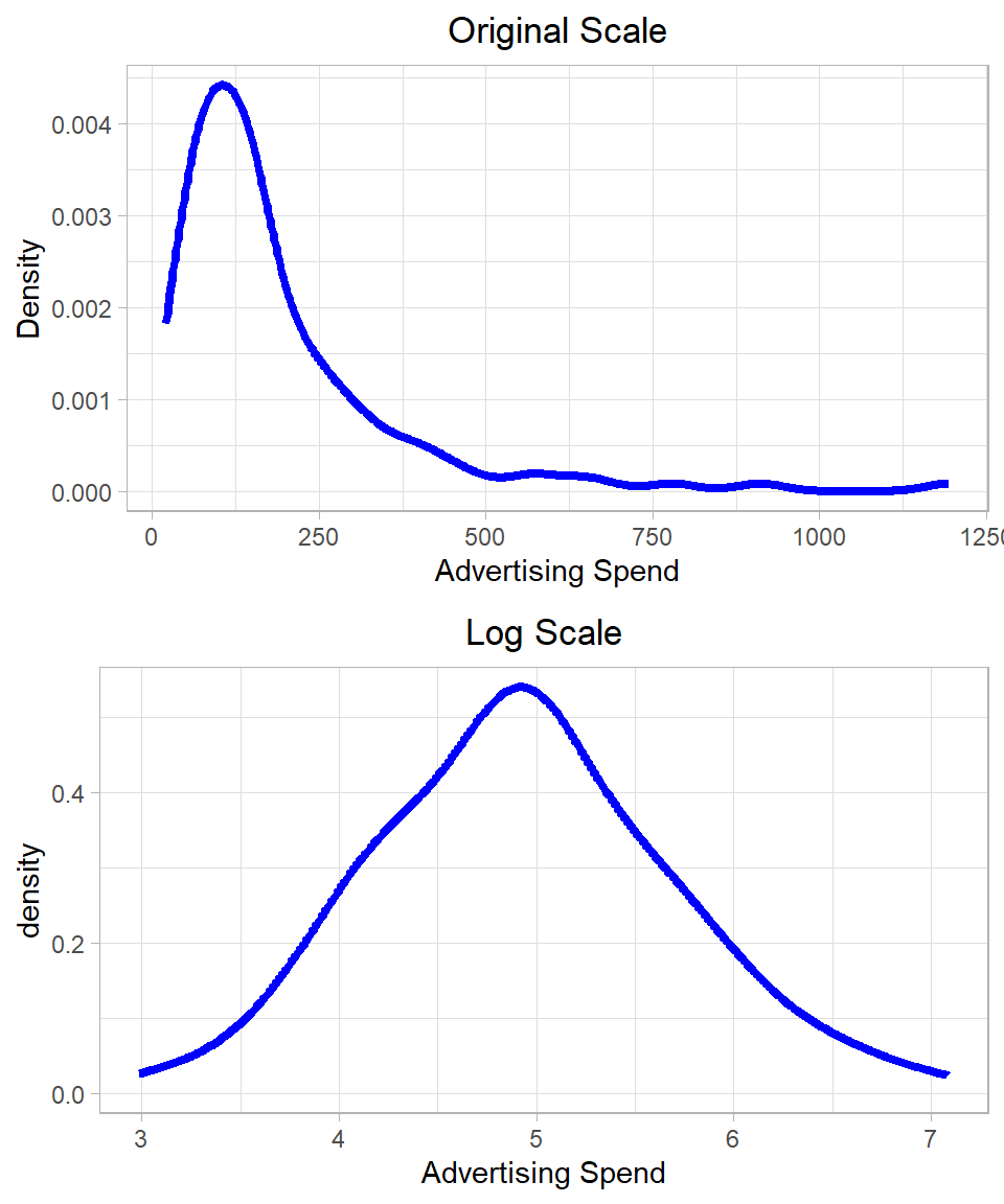
In our dataset, both the dependent variable Revenue and the independent variable Ad_Spend exhibit right-skewed distributions. These are characteristic of log-normal distributions, suggesting that a logarithmic transformation may help make the variables more symmetric and better suited for linear modeling. The plots below show the distribution of the variables Ad_Spend and Revenue before and after applying the log transformation:
Figure 26.2: Distribution of Revenue and Advertising Spend on original and log scales.
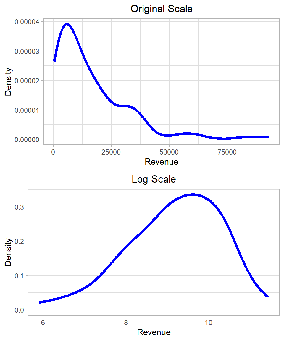
The following plots also illustrate how applying a logarithmic transformation can make it much easier to fit a linear model. On the left, we see the original variables, which show a nonlinear relationship. On the right, after taking the logarithm of both variables, the relationship appears much more linear, and the regression line fits the data more closely. This improved linearity is one reason why log transformations are commonly used in practice:
Figure 26.3: Linear regression using original and log scales.
We also observe that the log transformation reduces the influence of outliers. Extremely large values, which can disproportionately affect the regression estimates, become compressed on the log scale, thus stabilizing the estimation and improving model robustness.
However, we must exercise caution when applying a log transformation. Logarithms are only defined for positive numbers. If the variable contains zero or negative values, we either need to filter or shift the data appropriately (e.g., using log(x + 1)), or consider an alternative transformation. Arbitrary adjustments such as log(x + 1) must be justified carefully, as they affect the interpretation of the coefficients.
Let’s now apply a log-log transformation in R, where both the dependent and independent variables are logged before fitting the regression model:
# Fitting the linear regression model - log-loglm_model_log_log <-lm(log(Revenue) ~log(Ad_Spend), data = eshop_revenues)# Printing resultssummary(lm_model_log_log)
Call:
lm(formula = log(Revenue) ~ log(Ad_Spend), data = eshop_revenues)

Residuals:
    Min      1Q  Median      3Q     Max
-2.0535 -0.4439  0.0595  0.5966  1.5515

Coefficients:
              Estimate Std. Error t value             Pr(>|t|)
(Intercept)     4.0004     0.4602    8.69    0.000000000000015 ***
log(Ad_Spend)   1.0470     0.0921   11.37 < 0.0000000000000002 ***
---
Signif. codes:  0 '***' 0.001 '**' 0.01 '*' 0.05 '.' 0.1 ' ' 1

Residual standard error: 0.802 on 128 degrees of freedom
Multiple R-squared:  0.502, Adjusted R-squared:  0.498
F-statistic:  129 on 1 and 128 DF,  p-value: <0.0000000000000002
The estimated coefficient of log(Ad_Spend) is approximately 1.05 and statistically significant at the 1% level. This means that, on average, a 1% increase in advertising spend is associated with a 1.05% increase in revenue.
Interestingly, the R-squared and adjusted R-squared values have increased compared to the un-transformed model. While this may suggest a better fit, we should be cautious in interpreting such improvements across models with different scales. Log-transforming the dependent variable compresses the range of its values, making it easier to explain the variation. Hence, R-squared may appear artificially higher even if predictive performance does not improve on the original scale.
It is also worth noting that, even though we are applying linear regression, the log transformation means that we are modeling a nonlinear relationship in the original data. This is a subtle but important point: the regression model remains linear in the parameters but nonlinear in the variables.
In practice, the base of the logarithm (natural log, base-10, base-2, etc.) does not affect the qualitative results of the regression—it only rescales the coefficients. Most statistical packages, including R, use the natural logarithm (log with base e) by default. If we use a different base, the interpretation of the coefficients must be adjusted accordingly. For consistency and comparability across studies, the natural logarithm is generally preferred.
Adding Polynomial Terms
Another option to enhance a linear regression model is to include quadratic or higher-order polynomial terms. A quadratic term refers to squaring an independent variable and including that squared term as an additional independent variable in the model. This allows the model to capture nonlinear relationships—specifically, relationships that follow a curved (parabolic) pattern rather than a straight line.
Including a quadratic term changes the interpretation of the coefficients. In a model of the form:
\[y = \beta_0 + \beta_1 x_1 + \beta_2 x^2_1 + u\]
The coefficient \(\beta_1\) represents the marginal effect of advertising spend when Ad_Spend is zero.
The coefficient \(\beta_2\) captures the rate at which the marginal effect of Ad_Spend is changing.
Together, the model allows the relationship between advertising and revenue to bend either upward or downward, depending on the sign and magnitude of \(\beta_2\).
This added flexibility can improve model fit when the true relationship is nonlinear.
In R, we can include polynomial terms using the function I(), which prevents the ^ operator from being interpreted as a formula operator:
# Fitting the linear regression model with quadratic termlm_model_poly <-lm(Revenue ~ Ad_Spend +I(Ad_Spend^2), data = eshop_revenues)# Printing resultssummary(lm_model_poly)
Call:
lm(formula = Revenue ~ Ad_Spend + I(Ad_Spend^2), data = eshop_revenues)

Residuals:
   Min     1Q Median     3Q    Max
-27627  -5880  -2016   5768  44951

Coefficients:
                Estimate Std. Error t value         Pr(>|t|)
(Intercept)   -1866.5256  2138.8141   -0.87             0.38
Ad_Spend        120.6629    14.8427    8.13 0.00000000000033 ***
I(Ad_Spend^2)    -0.0727     0.0159   -4.58 0.00001109243713 ***
---
Signif. codes:  0 '***' 0.001 '**' 0.01 '*' 0.05 '.' 0.1 ' ' 1

Residual standard error: 11600 on 127 degrees of freedom
Multiple R-squared:  0.488, Adjusted R-squared:  0.48
F-statistic: 60.4 on 2 and 127 DF,  p-value: <0.0000000000000002
The model includes both a linear term (Ad_Spend) and a quadratic term (Ad_Spend^2) as predictors. The estimated regression equation is:
Both the linear and quadratic terms are statistically significant at the 1% level, with p-values well below 0.01. This provides strong evidence of a non-linear relationship between ad spend and revenue.
The interpretation of the coefficients is as follows:
The coefficient for Ad_Spend (120.66) indicates that, initially, increasing Ad_Spend leads to higher revenue—approximately 120.66 units for each additional unit of spending.
The negative coefficient for the quadratic term (–0.07) reflects diminishing returns: while advertising is beneficial at first, its impact decreases as spending rises. Eventually, the cost of additional advertising outweighs the benefit, and revenue starts to decline. This is common in business settings where saturation occurs. Beyond a certain point, customers have already been reached or are not influenced further, making extra ad spending inefficient.
Thus, 1-unit increase in Ad_Spend is associated with an increase of approximately 120.66 units in revenue, but this effect gradually decreases due to the negative quadratic term; at higher levels of Ad_Spend, the gains diminish and can even turn negative.
Adding a quadratic term often improves the goodness of fit, as measured by the R-squared and adjusted R-squared values. However, we must be careful: just because a model fits better numerically does not mean it is better conceptually or substantively.
Quadratic Terms with Log-Transformed Variables: Order Matters
If we are working with log-transformed variables and wish to include quadratic terms, we must be careful with the order of operations. Squaring the log-transformed variable log(Ad_Spend) is not the same as logging a squared variable. That is:
\[[\log(x)]^2 \ne \log(x^2)\]
Based on log properties:
\[\log(x^2) = 2 \cdot \log(x)\]
Whereas:
\[[\log(x)]^2 = \log(x) \cdot \log(x)\]
This distinction is important when building models. If we include both \(\log(x)\) and \(\log(x^2)\) in a regression, we are effectively including \(\log(x)\) and \(2 \cdot \log(x)\), which are apparently perfectly collinear. In such cases, R will automatically drop one of the terms to avoid multicollinearity and fit the model properly.
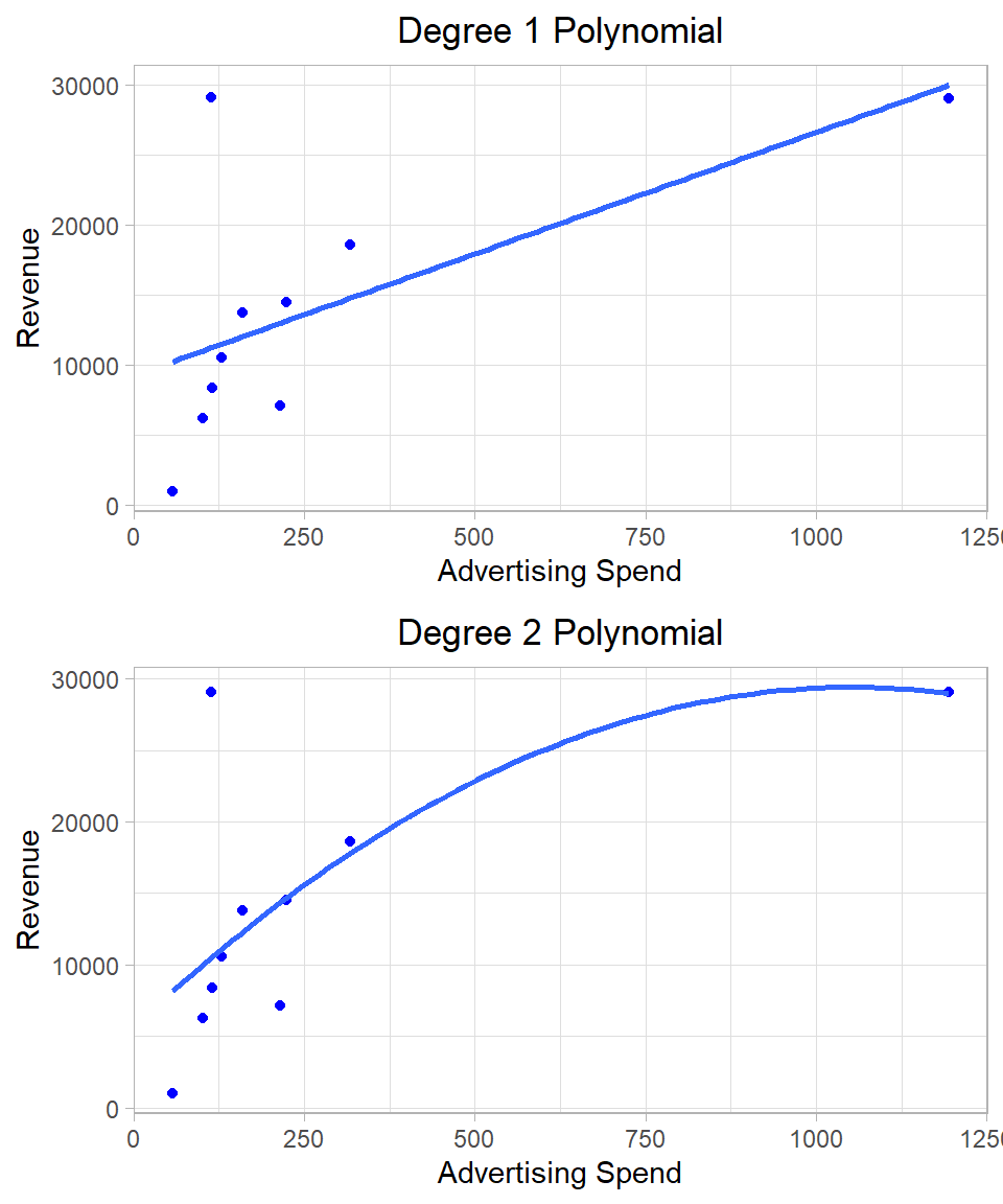
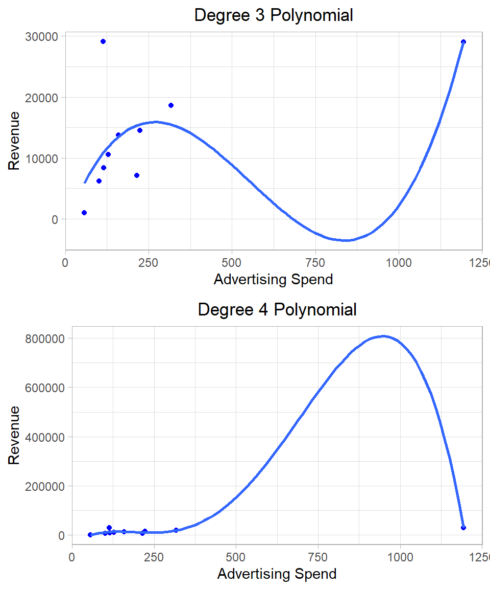
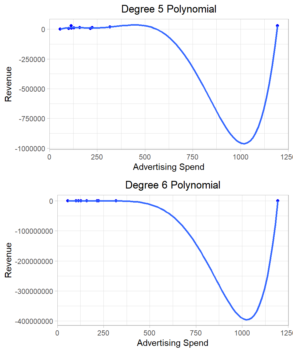
Introducing quadratic (and higher-order) terms increases the flexibility of the model, allowing it to capture more complex patterns in the data. In fact, if we keep adding polynomial terms—say, up to the 9th power with 10 data points—we can build a model that passes through every single point. However, such a model would be meaningless in most cases in terms of interpretation and statistical inference.
To illustrate this, consider a toy example using just the first 10 observations of our dataset. We can fit several models, starting from a simple linear regression model and add polynomial terms up to the 6th degree. The following plots show the data points and the regression lines separately:
Figure 26.4: Linear regression using different polynomial terms.
After a certain point (often after the quadratic or cubic term), adding more powers does not improve our understanding of the relationship. The coefficients become harder to interpret, and the model loses its explanatory power. Remember, our goal is not just to fit the data, but to produce unbiased, efficient estimates that are interpretable and support statistical inference. If we only cared about tracing a curve through every data point, there would be no need to worry about assumptions or inference.
Interaction Effects
So far, we’ve assumed that the effect of each independent variable on the dependent variable is additive, meaning each variable contributes to the outcome independently of the others. However, this is not always realistic. Sometimes, the effect of one variable depends on the level of another variable. In such cases, we include an interaction term in our model.
An interaction allows us to model the combined effect of two variables that goes beyond just adding their separate impacts. For example, imagine a company selling two types of products: basic and premium. The impact of a salesperson’s experience on sales might differ depending on the product type. For basic products, even a new salesperson might sell well because the product is simple, but for premium products, more experienced salespeople might be needed to close deals successfully. Here, the effect of experience on sales depends on the product type—this is an interaction. By including an interaction term between experience and product type in our regression model, we capture this nuanced relationship that neither variable alone can explain.
1. Interaction Effect with Dummy Variables
Let’s start with the simplest case: interactions between two dummy variables. A linear regression model with two dummy variables and their interaction effect can be written as:
The variables \(x_1\) and \(x_2\) are two dummy variables while the term \(x_1 \cdot x_2\) is the interaction term. The multiplication logic is straightforward: when both dummy variables are 1, their product is also 1, activating the interaction term. If either variable is 0, the product is 0, and the interaction term has no effect.
As an example, we will use two categorical variables: Price_Level (with four levels) and New_Product (a binary indicator: 1 if the product is new, 0 otherwise). Our goal is to see whether the effect of Price_Level on revenue differs depending on whether the product is new. To model this, we include both variables and their interaction term:
In R, we include interaction terms in the model using either asterisk (*) (which includes the main effects and the interaction) or colon (:) (which includes only the interaction):
# Fit a linear regression model with interaction effectlm(Revenue ~factor(Price_Level) * New_Product, data = eshop_revenues) %>%summary()
In the output, we see coefficients for all the dummy variable levels except the reference combination—in this case, Price_Level = 1 and New_Product = 0. This means the baseline group is existing products priced at level 1. The intercept captures the expected revenue for this reference group.
Binary Predictors as Factors
Because New_Product has only two values, it does not make any difference if we use it as a numeric or a factor variable in lm().
Additionally, we see three interaction effects, one for each of the three non-reference levels of Price_Level. These coefficients tell us how the revenue changes for new products relative to existing products at each price level.
The interaction effects can sometimes be tricky to interpret, but plugging in values makes them easier to understand. Here’s how to interpret each coefficient:
\(\beta_0 = 19,019\): This is the expected revenue when Price_Level = 1 and New_Product = 0 (i.e., an existing product at the baseline price level). It is statistically significant at the 1% level, indicating that this base revenue is reliably different from zero.
\(\gamma_1 = -478\): Among existing products, price level 2 is associated with a decrease of approximately 478 units in revenue compared to price level 1. This effect is not statistically significant different from 0 even at the 10% significance level, meaning we cannot confidently conclude that level 2 differs from level 1 for existing products.
\(\gamma_2 = -8,942\): Among existing products, price level 3 leads to a revenue reduction of about 8,942 units compared to level 1. This effect is statistically significant at the 10% significance level, suggesting a possible but not definitive difference.
\(\gamma_3 = -10,490\): For existing products, price level 4 is associated with a revenue drop of around 10,490 units compared to level 1. This coefficient is statistically significant at the 5% level, indicating that the effect is likely not due to chance.
\(\gamma_4 = -4,320\): For price level 1, new products generate about 4,320 units less revenue than existing products. However, this effect is not statistically significant different from 0 even at the 10% significance level, so we cannot confidently say that new and existing products differ in revenue at the baseline price level.
\(\gamma_5 = 14,726\): For new products at price level 2, revenue increases by approximately 14,726 units relative to what we would expect if we just added the individual effects of being in price level 2 and being a new product. In other words, this interaction “offsets” the negative effects of price level 2 and newness to bring the total effect closer to positive territory. Also, this term is statistically significant at the 10% significance level.
\(\gamma_6 = 17,585\): A similar interaction occurs at price level 3. For new products in this price category, revenue is adjusted upward by about 17,585 units compared to what we would expect from the main effects alone. Although the effect is strong in magnitude, it is not statistically significant different from 0 even at the 10% significance level.
\(\gamma_7 = 4,438\): For new products at price level 4, the interaction effect adds about 4,438 units in revenue, but again this adjustment is not statistically significant different from 0 even at the 10% significance level.
These results suggest that the revenue impact of introducing a new product depends on the price level. For example, while new products generally perform worse than existing ones at price level 1, this pattern changes at other price levels. In fact, the negative effect of introducing a new product is partially or completely offset by the interaction term at price levels 2 and 3. This kind of interaction modeling is useful when the effect of one variable depends on the level of another. Without the interaction term, we would have assumed that the effect of a new product is the same across all price levels—which the data does not seem to support.
2. Interaction Effect with Continuous and Dummy Variables
Another option is to include an interaction between a dummy variable and a continuous variable. In this case, the interaction does not just shift the intercept—it also implies a different slope for the continuous variable depending on the value of the dummy variable.
So, the intercept and the slope both change for new products. This lets us model a different relationship between ad spend and revenue for each product type.
For example, suppose we want to examine how Ad_Spend and New_Product jointly affect Revenue. It is reasonable to think that the impact of advertising may differ depending on whether a product is new or an existing one. To capture this possibility, we include an interaction term in the model:
If the interaction term is statistically significant, this would indicate that the relationship between Ad_Spend and Revenue depends on whether the product is new. For instance, advertising might generate a stronger increase in revenue for new products than for existing ones.
In R, we include this interaction in the same way using asterisk (*), which adds both main effects and the interaction:
# Fit a linear regression model with interaction effectlm(Revenue ~ Ad_Spend * New_Product, data = eshop_revenues) %>%summary()
Call:
lm(formula = Revenue ~ Ad_Spend * New_Product, data = eshop_revenues)

Residuals:
   Min     1Q Median     3Q    Max
-35299  -6449  -2311   5227  49375

Coefficients:
                     Estimate Std. Error t value       Pr(>|t|)
(Intercept)           5473.47    1753.46    3.12         0.0022 **
Ad_Spend                49.30       6.84    7.21 0.000000000045 ***
New_Product          -1254.88    3736.68   -0.34         0.7376
Ad_Spend:New_Product    38.59      14.32    2.70         0.0080 **
---
Signif. codes:  0 '***' 0.001 '**' 0.01 '*' 0.05 '.' 0.1 ' ' 1

Residual standard error: 12000 on 126 degrees of freedom
Multiple R-squared:  0.458, Adjusted R-squared:  0.446
F-statistic: 35.6 on 3 and 126 DF,  p-value: <0.0000000000000002
The interpretation of this output is the following:
\(\beta_0 = 5,473.47\): This is the expected revenue when Ad_Spend = 0 for existing products (New_Product = 0). It is statistically significant at the 1% level, indicating that this base revenue is reliably different from zero.
\(\beta_1 = 49.30\): For existing products, 1-unit increase in Ad_Spend is associated with a revenue increase of about 49.3 units, a statistically significant effect at the 1% significance level.
\(\gamma_1 = -1,254.88\): When Ad_Spend = 0, new products have lower revenue than existing products by approximately 1,255 units, but this difference is not statistically significant even at the 10% significance level.
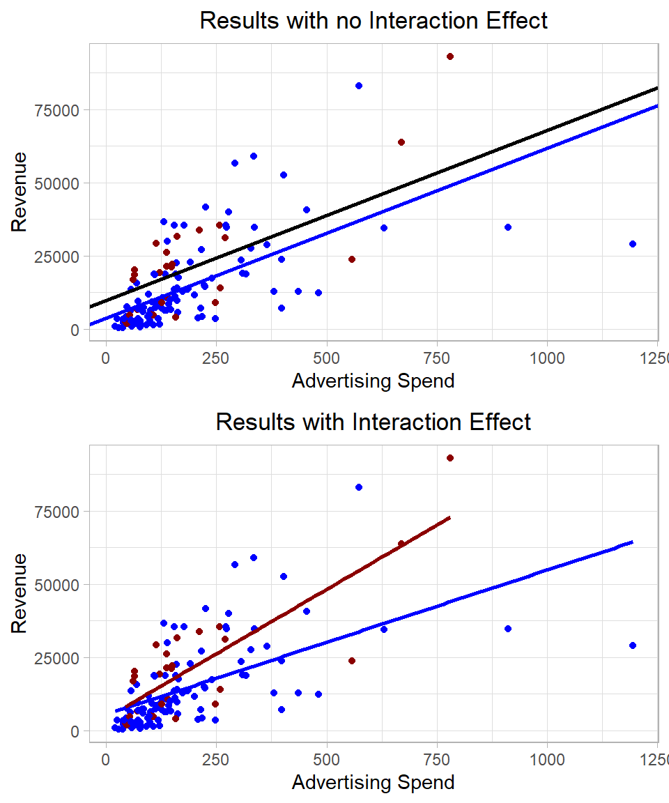
\(\beta_2 = 38.59\): For new products, the slope of ad spend increases by 38.59 units compared to existing products. This means new products are more responsive to ad spend. The total slope for new products is 49.30 + 38.59 = 87.89, and this interaction effect is statistically significant at the 1% level.
To visualize how the slopes differ by product type, we can plot two regression lines, one for new products and one for existing products:
Figure 26.5: Linear regression including interaction and no interaction terms.
So, including an interaction between a dummy variable and a continuous variable allows the regression to estimate different slopes for each group. In fact, this is mathematically equivalent to fitting a separate linear regression model for each group. However, by including the interaction within a single model, we keep everything unified, making it easier to compare groups directly and test whether the differences in slopes and intercepts are statistically significant.
This unified approach has several advantages:
Smaller Standard Errors: When we estimate separate models for each group, each model uses only a portion of the data, which can lead to larger standard errors, especially if group sizes are small. By pooling the data into a single model with interaction terms, we make more efficient use of the data, which often results in smaller standard errors and more reliable estimates.
Better Overall Significance Testing: A combined model lets us test joint hypotheses across groups, such as whether the slope is truly different between groups or whether both groups share the same intercept. This would not be as straightforward if we estimated separate models.
Model Efficiency and Parsimony: Including interaction terms in one model avoids duplicating effort across multiple models. It’s computationally and conceptually cleaner, especially when extending to more than two groups or adding further predictors.
Improved Interpretation: A single model makes it easier to interpret how a continuous variable behaves across different groups by directly comparing estimated slopes and intercepts, along with their confidence intervals and p-values.
In short, a model with interaction terms captures group-specific effects while leveraging the full dataset, leading to more precise estimates and more informative statistical inference.
3. Interaction Effect with Continuous Variables
Including the interaction effect between two continuous variables is also possible and often useful when we suspect that the relationship between one predictor and the outcome depends on the level of another predictor. In this case, the interaction does not simply shift the intercept or change the slope in a fixed way for a group—it creates a continuously varying effect that depends on the values of both variables.
where \(x_1\) and \(x_2\) are two continuous variables. The coefficients \(\beta_1\) and \(\beta_2\) capture the main effects of these variables while the coefficient \(\beta_3\) captures the interaction effect.
As an example, suppose we are interested in how Ad_Spend and Website_Visitors together affect Revenue. We might think that the effectiveness of ad spend depends on how many visitors are already coming to the site (or vice versa). Then, our model becomes:
If the interaction term is statistically significant, this suggests that the relationship between Ad_Spend and Revenuedepends on the number of Website_Visitors. For example, advertising may be more effective when website traffic is already high, and so the combined effect is more than additive.
To estimate this interaction in R, we still use the asterisk (*) inside the lm() function:
# Fitting a linear regression model with interaction effectlm(Revenue ~ Ad_Spend * Website_Visitors, data = eshop_revenues) %>%summary()
Call:
lm(formula = Revenue ~ Ad_Spend * Website_Visitors, data = eshop_revenues)

Residuals:
   Min     1Q Median     3Q    Max
-33824  -6069  -2360   6078  44907

Coefficients:
                             Estimate  Std. Error t value Pr(>|t|)
(Intercept)               -15881.3842   6031.9586   -2.63  0.00953 **
Ad_Spend                      92.1460     26.8436    3.43  0.00081 ***
Website_Visitors              18.7583      5.0786    3.69  0.00033 ***
Ad_Spend:Website_Visitors     -0.0293      0.0173   -1.70  0.09218 .
---
Signif. codes:  0 '***' 0.001 '**' 0.01 '*' 0.05 '.' 0.1 ' ' 1

Residual standard error: 12000 on 126 degrees of freedom
Multiple R-squared:  0.462, Adjusted R-squared:  0.449
F-statistic:   36 on 3 and 126 DF,  p-value: <0.0000000000000002
The interpretation of this output is the following:
\(\beta_0 = -15,881.38\): This is the estimated revenue when both Ad_Spend = 0 and Website_Visitors = 0. While this specific combination may not be realistic in practice, the intercept serves as a baseline reference. It is statistically significant at the 1% level.
\(\beta_1 = 92.15\): When the number of website visitors is held constant, a 1-unit increase in Ad_Spend is associated with an average increase of 92.15 units in revenue. This effect is statistically significant at the 1% level, indicating that advertising spend has a meaningful positive impact on revenue.
\(\beta_2 = 18.76\): When Ad_Spend is held constant, an additional website visitor is associated with an average increase of 18.76 units in revenue. This effect is also statistically significant at the 1% level, showing that website traffic positively contributes to revenue.
\(\beta_3 = -0.03\): This is the interaction effect between Ad_Spend and Website_Visitors. It indicates that the marginal effect of Ad_Spend decreases slightly as the number of website visitors increases, and vice versa. Specifically, for every additional website visitor, the effect of Ad_Spend on revenue decreases by 0.029 units. This interaction effect is statistically significant at the 10% significance level, suggesting some evidence that the impact of one predictor may depend on the level of the other.
In summary, including an interaction between two continuous variables allows the model to capture situations where the effect of one variable depends on the level of another. While these interactions can offer richer insights, they also require careful interpretation. To highlight the value of the Chow test, we add three more independent continuous variables into the model: Website_Visitors, Product_Quality_Score and Customer_Satisfaction.
4. Other Interaction Effects
Apart from the cases we discussed, nothing prevents us from using interaction effects in combination with transformed variables, such as logarithms or quadratic terms, or even creating interaction terms involving more than two variables. These extensions allow us to capture more nuanced relationships in the data, especially when the effect of one variable may depend on both the level and the rate of change of another.
For example, we might include an interaction between a dummy variable and a log-transformed continuous variable if we suspect diminishing returns for one group but not another. Alternatively, interacting a quadratic term (e.g., x^2) with another variable can help us capture group-specific nonlinear effects. Similarly, three-way interactions like x1 * x2 * x3 allow us to examine how the joint influence of two variables varies depending on a third—though interpretation quickly becomes more complex.
The main trade-off is interpretability versus flexibility. As we add more interaction terms, especially nonlinear or higher-order ones, the model becomes more flexible and capable of fitting subtle patterns in the data. However, this also increases complexity, especially in smaller datasets. Moreover, interpreting interaction effects beyond two variables often requires visual aids or marginal effects plots, as the coefficients alone can become difficult to unpack. So while the expressiveness of the model grows, so does the need for care in interpretation and validation.
It is rare in practice to use such complicated interaction effects, especially if the goal is interpretation. As models become more complex, the coefficients become harder to explain, and the risk of misinterpreting the relationships increases. In applied work—particularly in business, economics, and the social sciences—models are often judged not only by their predictive accuracy but also by how clearly they communicate insights. Adding multiple or nonlinear interaction terms may obscure rather than clarify the story the data is telling.
Why Main Effects Should Accompany Interaction Terms
One interesting question is whether we can include only the interaction terms in a linear regression model, without the main effects. While this is technically possible, it is generally not recommended. The main effects represent the individual contribution of each predictor, whereas interaction terms capture how the predictors combine to influence the outcome. Omitting the main effects can make the model harder to interpret and may lead to misleading conclusions, as the interaction terms no longer reflect deviations from the additive effects of the individual variables. For this reason, it is good practice to include the main effects whenever interaction terms are added.
Putting Everything Together
Before we wrap up this chapter, let’s bring everything together by fitting a more complete linear regression model. This will help us see how multiple variables and their relationships interact in practice.
We will run a linear regression model on Revenue, using the following predictors:
log(Ad_Spend) to account for diminishing returns from advertising
Website_Visitors and its squared term to allow for a non-linear relationship
Product_Quality_Score and Customer_Satisfaction, along with their interaction, to capture product and service characteristics
New_Product, along with their interaction, to account for how pricing might work differently depending on whether the product is new
We will interpret the value of each coefficient, assess its statistical significance, comment on the overall significance of the model, and test for heteroskedasticity. Lastly, we will perform a joint significance test on a pair of coefficients.
We will interpret the value of each coefficient, assess its statistical significance, comment on the overall significance of the model, and test for heteroskedasticity. Lastly, we will perform a joint significance test on the coefficients of Product_Quality_Score, Customer_Satisfaction and their interaction effect to see whether they collectively have a meaningful effect on the outcome.
We can fit this model in R using the following code:
# Fitting a final linear regression modellm_final_model <-lm(Revenue ~log(Ad_Spend) + Website_Visitors +I(Website_Visitors^2) + Product_Quality_Score * Customer_Satisfaction + New_Product,data = eshop_revenues)# Printing the resultslm_final_model %>%summary()
The interpretation of each coefficient is as follows:
\(\beta_0 = -21,163.75\): This is the estimated revenue when all predictors are zero. While this scenario may not be realistic, the intercept serves as the baseline level of the regression surface. It is statistically significant at the 1% level, indicating that this base level is reliably different from zero.
\(\beta_1 = 11,531.97\): A 1% increase of Ad_Spend is associated with an increase of approximately 115.32 units in Revenue, holding other variables fixed. This effect is statistically significant at the 1% significance level, showing a strong and positive relationship between advertising and revenue.
\(\beta_2 = -42.34\): Each additional website visitor is associated with a decrease of 42.34 units in revenue, holding other variables constant. This may seem counterintuitive, but we must interpret it together with the squared term below, as the relationship is nonlinear. The coefficient is statistically significant at the 5% level.
\(\beta_3 = 0.02\): This is the coefficient for the squared term of Website_Visitors. It is positive and statistically significant at the 5% significance level, suggesting that the effect of visitors on revenue becomes more positive (or less negative) as the number of visitors increases. This implies a U-shaped relationship: revenue initially decreases with more visitors but then starts increasing at higher levels.
\(\beta_4 = -5,134.25\): A one-unit increase in the Product_Quality_Score is associated with a decrease in revenue when customer satisfaction is held constant at zero. However, this coefficient is not statistically significant even at the 10% significance level, and must also be interpreted alongside its interaction with customer satisfaction.
\(\beta_5 = -2,497.92\): A one-unit increase in Customer Satisfaction is associated with a decrease in revenue when product quality score is zero. Again, this is not statistically significant even at the 10% significance level, and its standalone interpretation is limited due to the interaction term.
\(\gamma_1 = 4,545.25\): New products are associated with an average increase in revenue of about 4,545 units compared to existing products, holding other factors fixed. This effect is statistically significant at the 5% level.
\(\beta_6 = 1,029.18\): This is the interaction between Product_Quality_Score and Customer_Satisfaction. It indicates how the combined effect of these two variables influences revenue. Although this interaction term is not statistically significant at the 5% level, its magnitude suggests that when both quality and satisfaction increase together, their joint effect may be positive.
In terms of model fit, R-squared and adjusted R-squared are both between 60% and 65%, suggesting a strong fit of the model. The p-value of the overall significance is lower than 0.01, suggesting that the model as a whole explains a significant portion of the variation in revenue and that at least one of the predictors is meaningfully related to the outcome.
This model reveals strong evidence for the positive effect of advertising and some evidence that new products perform better. While the individual effects of quality and satisfaction are not significant alone, their combined interaction might still be practically important and worth exploring further.
To make a rigorous assessment of whether heteroskedasticity is present in our regression model, we will use the F-version of the Breusch-Pagan test. This test examines whether the variance of the residuals depends systematically on one or more explanatory variables, which would violate the assumption of constant variance (homoskedasticity) required for standard inference (see Chapter Linear Regression - Statistical Inference).
Here is how we implement the test in R:
# Extracting residuals and square themu <- lm_final_model %>%residuals()u_squared <- u^2# Auxiliary regression: squared residuals on original predictorslm(u_squared ~log(Ad_Spend) + Website_Visitors +I(Website_Visitors^2) + Product_Quality_Score * Customer_Satisfaction + New_Product, data = eshop_revenues) %>%summary()
If the p-value from this auxiliary regression is below 0.01, as in our case, it indicates strong evidence of heteroskedasticity, meaning the residual variance changes with the predictors.
To make more valid statistical inferences despite heteroskedasticity, we need to use heteroskedasticity-robust standard errors. This allows us to trust our hypothesis tests and confidence intervals without the homoskedasticity assumption.
Here is the R code for computing robust standard errors and testing coefficients:
# Librarieslibrary(sandwich)library(lmtest)# Calculating robust standard errorsrobust_se <-vcovHC(lm_final_model, type ="HC1")# Performing coefficient tests with robust standard errorscoeftest(lm_final_model, vcov = robust_se)
After applying robust standard errors, we observe that the p-values for both the main effect and the quadratic effect of Website_Visitors have increased and are now statistically insignificant. This suggests that the initial significance we observed may have been influenced by heteroskedasticity, and the robust standard errors provide a more reliable inference in this case.
Even with heteroskedasticity present, linear hypothesis testing remains valid if we use robust standard errors. This ensures the test statistics follow the correct distribution under the null hypothesis, allowing us to perform reliable inference despite the violation of constant variance. We want to test whether the coefficients of the variables Product_Quality_Score, Customer_Satisfaction, and their interaction effect are jointly equal to zero.
While the individual t-tests for these coefficients suggest they are not statistically significant on their own, the joint test can reveal whether the combination of these variables has a meaningful effect on Revenue. This is because even if individual effects are weak, their combined influence might still be important.
The p-value from this F-test is much lower than 0.01, implying that collectively these variables significantly contribute to explaining the variation in Revenue. This contrasts with the individual coefficient tests, emphasizing the importance of testing joint hypotheses when variables are related or interact.
Recap
In this chapter, we discussed some advanced topics in linear regression, focusing on how to extend the basic model to better capture complex relationships in the data. We introduced non-linear components, such as logarithmic transformations and quadratic terms, and examined how these change the interpretation of coefficients. We also explored interaction effects, both between continuous variables and between continuous and categorical variables, to allow for relationships that vary across groups.
Throughout the chapter, we emphasized the importance of careful interpretation as models become more complex. Lastly, we built a comprehensive linear regression model that incorporated several of these extensions, interpreted its coefficients, tested for heteroskedasticity, and applied heteroskedasticity-robust standard errors to support valid statistical inference. This final example illustrated how all the individual techniques can be combined in practice to produce a richer and more reliable model.