# Libraries
library(tidyverse)

# Import the dataset
eshop_revenues <- read_csv("https://raw.githubusercontent.com/DataKortex/Data-Sets/refs/heads/main/eshop_revenues.csv")Multiple Linear Regression
Introduction
Multiple Linear Regression is a natural extension of Simple Linear Regression. While Simple Linear Regression models the relationship between one independent variable and one dependent variable, Multiple Linear Regression allows us to include two or more independent variables in our model. This enables us to better explain the variation in the outcome by considering multiple factors at once.
Simple Linear Regression can be quite limited—especially when we consider assumptions such as the Zero Conditional Mean. In real-world data, it’s often unrealistic to believe that all omitted factors are uncorrelated with the single independent variable. By including more relevant variables in the model, we reduce the risk of omitted variable bias and get closer to estimating causal relationships. This is where the idea of ceteris paribus—“all else equal”—becomes important. Multiple Linear Regression allows us to isolate the effect of one variable on the dependent variable while holding others constant.
Including more independent variables also means we now estimate more coefficients. In this chapter, we will explore how to derive these OLS estimates in the multiple regression context, how to interpret them, and how the key assumptions change or extend from the simple regression case. We’ll also discuss potential pitfalls, such as multicollinearity, and highlight the continued importance of careful model specification.
From Simple Linear Regression to Multiple Linear Regression
To begin, let’s reload our R environment by importing the necessary package and loading our dataset eshop_revenues:
A Multiple Linear Regression model takes the following form:
\[y = \beta_{0} + \beta_{1}x_{1} + \beta_{2}x_{2} + u\]
In this model, we still have one dependent variable, \(y\), and an error term, \(u\), just like in Simple Linear Regression. The difference is that we now include two independent variables, \(x_1\) and \(x_2\), each with its own coefficient, \(\beta_1\) and \(\beta_2\). These coefficients represent the effect of each independent variable on the dependent variable, holding the other variable fixed.
This is what allows us to make ceteris paribus interpretations. That is, we can isolate the effect of one variable while keeping all others fixed. For instance, suppose \(y\) represents Revenue, \(x_1\) is Ad_Spend, and \(x_2\) is a Product_Quality_Score. Then the multiple regression model is:
\[\hat{y} = \hat{\beta}_{0} + \hat{\beta}_{1} x_{1} + \hat{\beta}_{2} x_{2}\]
This model allows us to interpret the coefficients as follows:
If \(\hat{\beta}_1 = 30\), then a one-unit increase in \(x_1\) (
Ad_Spend) leads to a 30-unit increase in \(y\) (Revenue), holding \(x_2\) (Product_Quality_Score) constant:\[\Delta{y} = 30 \cdot \Delta{x}_{1}, \ \text{when} \ \Delta{x}_{2} = 0\]
If \(\hat{\beta}_2 = 0.5\), then a one-unit increase in \(x_2\) (
Product_Quality_Score) leads to a 0.5-unit increase in \(y\) (Revenue), holding \(x_1\) (Ad_Spend) constant:\[\Delta{y} = 0.5 \cdot \Delta{x}_{2}, \ \text{when} \ \Delta{x}_{1} = 0\]
These expressions highlight how we can interpret the coefficients independently of each other by isolating the effect of one variable while holding the others fixed. This is the essence of ceteris paribus reasoning in multiple regression.
Like in the simple linear regression case, there is a Population Regression Function that we aim to estimate. However, in practice, we do not know the true values of the coefficients \(\beta_{0}, \beta_{1}, \beta_{2}, \dots, \beta_{k}\). Instead, we use data to estimate them through the Ordinary Least Squares (OLS) method, obtaining the estimates \(\hat{\beta}_{0}, \hat{\beta}_{1}, \hat{\beta}_{2}, \dots, \hat{\beta}_{k}\).
We can include multiple independent variables in the model, allowing us to control for various factors that may influence the dependent variable. That said, as we will discuss later, there are practical and statistical limits to how many variables we can include. In general, a multiple linear regression model with \(k\) independent variables can be written as:
\[y = \beta_{0} + \beta_{1} x_{1} + \beta_{2} x_{2} + ... + \beta_{k} x_{k} + u\]
Visualizing the Linear Regression Line
In multiple linear regression, visualizing the results is generally impossible beyond three dimensions. However, when we have only two independent variables, we can still create meaningful visualizations.
In the plot below, Ad_Spend is on the x-axis and Revenue is on the y-axis. The blue line represents the regression line from a simple linear regression of Revenue on Ad_Spend only. The red line, on the other hand, represents the fitted values from the multiple linear regression where we regress Revenue on both Ad_Spend and Product_Quality_Score. To show the red line in two dimensions, we hold Product_Quality_Score fixed at its mean value. This allows us to isolate the effect of Ad_Spend while controlling for the quality score.
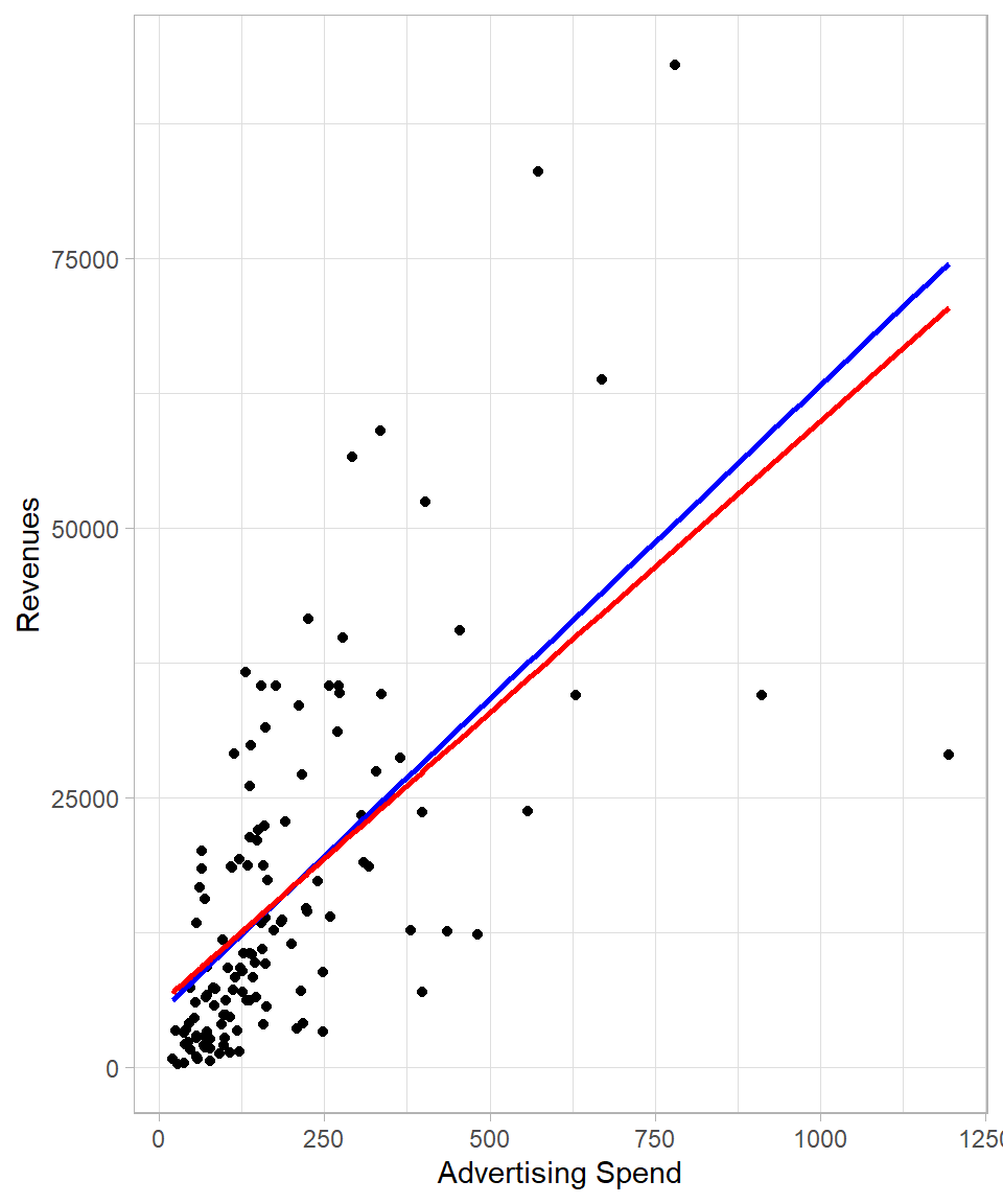
The blue line is actually the best fit in this two-dimensional plot, but it ignores the variation explained by Product_Quality_Score. The red line reflects the adjusted slope of Ad_Spend when we control for the other variable in the model. This shift in the slope happens because the coefficient \(\hat{\beta}_1\) changes when we account for the second variable, capturing the effect of Ad_Spend ceteris paribus.
To better understand how the multiple regression works in three dimensions, we can visualize the regression plane. In the next plot, we display a 3D surface that shows how Revenue changes with both Ad_Spend and Product_Quality_Score. Each point represents an observation, and the red plane is the best linear fit across both predictors:
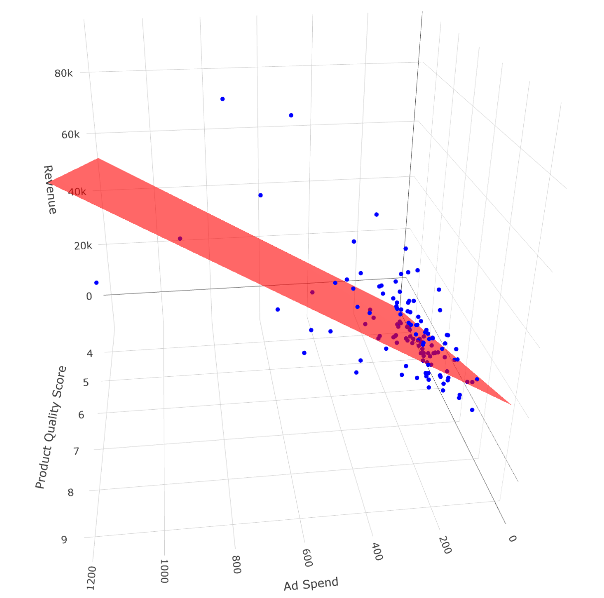
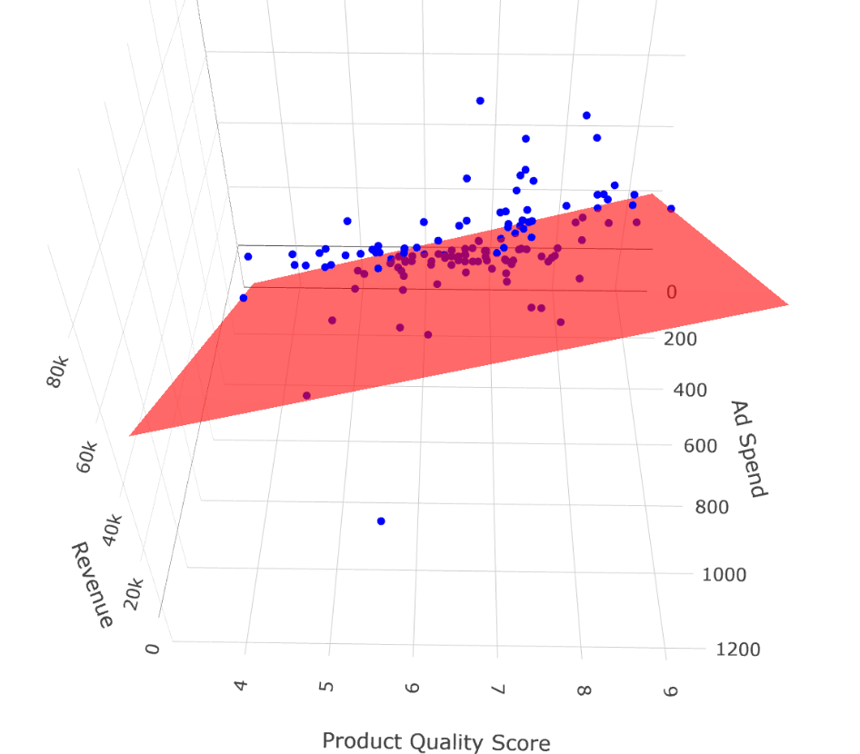
These 3D visualizations provide a more complete but more complicated picture of the regression model, showing how both predictors simultaneously influence the dependent variable. Specifically, the second plot shows when both predictor increase, the expected value of the dependent variable also increases. Additionally, for a fixed level of Product_Quality_Score (e.g., a value of 8), the higher the Ad_spend, the higher the expected value of Revenue; this is exactly what we mean by ceteris paribus.
Deriving Coefficients with OLS
To derive the OLS coefficients in multiple linear regression, we once again rely on the Zero Conditional Mean assumption:
\[E(u | x_{1}, x_{2}, ... x_{k}) = E(u | \mathbf{X}) = 0\]
Here, \(\mathbf{X}\) is a matrix containing all the independent variables. A helpful way to think about this is that \(\mathbf{X}\) is just the data frame of the dataset with only the independent variables.
From the Zero Conditional Mean assumption, the error term is unrelated to any of the independent variables in the model. It implies that each independent variable is uncorrelated with the error term:
\[Cov(u, x_{1}) = 0, \ \ Cov(u, x_{2}) = 0, \ \ ..., \ \ Cov(u, x_{k}) = 0\]
Or, in summation form:
\[\sum^n_{i = 1} x_{ij} u_{i} = 0\]
where \(j = 0, 1, 2, ..., k\) and \(x_{i0}\) represents the intercept.
Now, recall the regression model:
\[y_{i} = \beta_0 + \beta_{1} x_{i1} + \beta_{2} x_{i2} + ... + \beta_{k} x_{ik} + u_{i}\]
Solving for \(u_{i}\), we have:
\[u_{i} = y_{i} - \beta_{0} - \beta_{1} x_{i1} - \beta_{2} x_{i2} - ... - \beta_{k} x_{ik}\]
Here, \(u_{i}\) represents the unobserved error term, which we cannot directly observe. To estimate the coefficients using OLS, we work with the residuals \(\hat{u}_i\) which measure the difference between the observed values and the fitted values from the regression:
\[\hat{u}_{i} = y_{i} - \hat{\beta}_{0} - \hat{\beta}_{1} x_{i1} - \hat{\beta}_{2} x_{i2} - ... - \hat{\beta}_{k} x_{ik}\]
Plugging this into our covariance condition gives us a system of \(k+1\) normal equations:
- For the intercept (where \(x_{i0} = 1\)):
\[\sum^n_{i = 1} \left ( y_{i} - \hat{\beta}_{0} - \hat{\beta}_{1} x_{i1} - \hat{\beta}_{2} x_{i2} - ... - \hat{\beta}_{k} x_{ik} \right ) = 0\]
For each independent variable:
\[\sum^n_{i = 1} x_{ij} \left ( y_{i} - \hat{\beta}_{0} - \hat{\beta}_{1} x_{i1} - \hat{\beta}_{2} x_{i2} - ... - \hat{\beta}_{k} x_{ik} \right ) = 0\]
In expanded form, the system of equations becomes:
\[\sum^n_{i = 1} \left ( y_{i} - \hat{\beta}_{0} - \hat{\beta}_{1} x_{i1} - \hat{\beta}_{2} x_{i2} - ... - \hat{\beta}_{k} x_{ik} \right ) = 0\]
\[\sum^n_{i = 1} x_{i1} \left ( y_{i} - \hat{\beta}_{0} - \hat{\beta}_{1} x_{i1} - \hat{\beta}_{2} x_{i2} - ... - \hat{\beta}_{k} x_{ik} \right ) = 0\]
\[\sum^n_{i = 1} x_{i2} \left ( y_{i} - \hat{\beta}_{0} - \hat{\beta}_{1} x_{i1} - \hat{\beta}_{2} x_{i2} - ... - \hat{\beta}_{k} x_{ik} \right ) = 0\]
\[...\]
\[\sum^n_{i = 1} x_{ik} \left ( y_{i} - \hat{\beta}_{0} - \hat{\beta}_{1} x_{i1} - \hat{\beta}_{2} x_{i2} - ... - \hat{\beta}_{k} x_{ik} \right ) = 0\]
Solving this system gives the OLS estimates for the coefficients. While the solution involves linear algebra or multivariable calculus, we usually let software like R handle the math for us. It is crucial to note, though, that the number of restrictions we get is directly related to the number of independent variables we include in the model. Each variable adds one equation (or restriction) through the zero conditional mean assumption. However, if we include more variables (columns) than data points (rows), the system becomes unsolvable—the matrix of independent variables loses full rank, and OLS cannot compute unique coefficient estimates. Intuitively, this means we are trying to estimate more unknowns than we have information to determine them: there simply isn’t enough data to pin down a unique solution.
The key point is the logic: the coefficients are chosen so that the residuals are uncorrelated with all the independent variables. In other words, once we’ve accounted for the predictors in the model, what’s left (the error) shouldn’t be related to any of them (Montgomery, Peck & Vining, 2021; Greene, 2018).
So, while the multiple regression case involves more equations, the underlying principle is exactly the same as in simple linear regression.
Calculating in R and Interpreting the Results
To fit a multiple linear regression model, we again use the lm() function with the tilde sign ~ to separate the dependent variable from the independent variables. To include more than one predictor, we simply add them using the + sign. As with simple linear regression, the object created by the lm() function stores much more than just the coefficients, such as the fitted (predicted) values and the residuals).
Let’s create a linear regression model using the dataset we imported:
# Fitting a linear regression model
lm_model <- lm(Revenue ~ Ad_Spend + Product_Quality_Score, data = eshop_revenues)

# Printing coefficients
print(lm_model)
Call:
lm(formula = Revenue ~ Ad_Spend + Product_Quality_Score, data = eshop_revenues)

Coefficients:
          (Intercept)               Ad_Spend  Product_Quality_Score
            -29861.84                  54.11                5427.83
This output includes the intercept as well as the coefficients for the variables Ad_Spend and Product_Quality_Score. Based on this output, the estimated regression equation is:
\[\widehat{\text{Revenue}}_{i} = -29861.84 + 54.11 \text{AdSpend}_{i} + 5427.83\text{ProductQualityScore}_{i}\]
The interpretation of the estimated coefficients is as follows:
\(\hat{\beta}_0 = -29,861.84\): This is the expected revenue when both
Ad_SpendandProduct_Quality_Scoreare equal to zero. In this context, that interpretation doesn’t make much sense as zero advertising and zero product quality are not realistic business scenarios, and revenue can’t reasonably be negative. Still, this value is part of the mathematical solution that minimizes the sum of squared residuals. The intercept ensures the regression plane is positioned optimally to best fit the data points overall. In many cases, especially when zero values of the independent variables fall outside the range of the observed data, the intercept has no meaningful real-world interpretation, but it is still necessary for the accuracy of the model. We should not ignore it in the regression equation, but we can avoid attaching practical meaning to it when it’s clearly unrealistic.\(\hat{\beta}_1 = 54.11\): This tells us that when
Ad_Spendincreases by 1 unit,Revenueis expected to increase by 54.11 units holdingProduct_Quality_Scorefixed. When we interpret coefficients in multiple regression, we always do so holding all other variables fixed.\(\hat{\beta}_2 = 5,427.83\): Similarly, a one-unit increase in
Product_Quality_Scoreis associated with an increase of approximately €5,428 inRevenue, holdingAd_Spendfixed.
In Chapter Simple Linear Regression, the coefficient for Ad_Spend was different, and we saw this in previous plot when we compared the regression lines with and without Product_Quality_Score. Why did the slope change?
This happens because, in multiple regression, each coefficient captures the partial effect of its variable on the dependent variable, controlling for all other variables in the model. In simple regression, the effect of Ad_Spend also absorbs any indirect effects that are actually due to other omitted variables such as Product_Quality_Score. So when we add more variables, the slope for Ad_Spend may change to account for the presence of this new information.
In this example, these estimated coefficients seem logical. We would expect that increasing the Product_Quality_Score would significantly boost revenues—after all, better products are more likely to attract and retain customers. The same applies to Ad_Spend: higher advertising investment tends to increase awareness and sales, leading to higher revenue. The coefficients also make sense from a magnitude perspective. A one-unit increase in product quality is associated with a substantial increase in revenue, while the effect of advertising spend is also positive but more moderate, reflecting the fact that both product quality and advertising contribute to revenue, albeit in different ways. This alignment between the model output and our real-world expectations gives us more confidence in these regression results.
Statistical Properties
The statistical properties of multiple linear regression are essentially the same as those of simple linear regression. Below are the key properties that hold under the standard OLS assumptions:
Sum of residuals is zero
The residuals from the regression always sum to zero. This ensures that, on average, the predicted values are not systematically above or below the actual values.
Sample covariance between each independent variable and the residuals is zero
After fitting the model, the residuals are uncorrelated with each of the independent variables. This property follows from the OLS estimation procedure, which minimizes the sum of squared residuals.
The regression line passes through the average values of the variables:
The fitted regression line (or plane, in higher dimensions) always passes through the point defined by the mean of the dependent variable and the means of the independent variables.
Decomposition of total variation:
The total variation in the dependent variable (Total Sum of Squares, TSS) can be decomposed into two parts: the explained variation (Explained Sum of Squares, ESS) and the unexplained variation (Residual Sum of Squares, RSS). That is:
\[\text{TSS} = \text{ESS} + \text{RSS}\]
Goodness-of-fit
R-squared (\(R^2\)) measures the proportion of the total variation in the dependent variable that is explained by the independent variables. While a higher \(R^2\) suggests a better fit, it has important limitations.
One key issue is that \(R^2\) never decreases when new variables are added to the model, even if those variables are completely unrelated to the dependent variable. This happens because both ESS and TSS either increase or stay the same, which mechanically inflates or preserves the value of \(R^2\).
This means \(R^2\) can be misleading when used to judge model quality or compare models with different numbers of predictors. A model might appear to fit better simply because it has more variables, not because those variables are useful. Another problem is that \(R^2\) is a biased estimate of model fit, especially in small samples.
To address the limitations of \(R^2\), especially its tendency to increase mechanically as more variables are added to the model, we often use the adjusted R-squared (\(\bar{R}^2\)). This version of the statistic introduces a correction for the number of predictors by accounting for degrees of freedom. Specifically, it replaces the raw sums of squares (RSS and TSS) in the \(R^2\) formula with their mean squares:
\[\bar{R}^2 = 1 - \frac{\text{RSS} / (n - k - 1)}{\text{TSS} / (n - 1)}\]
Here, \(n\) is the number of observations, and \(k\) is the number of independent variables (excluding the intercept). This adjustment means that \(\bar{R}^2\) can decrease if the added variables do not improve the model enough to justify the loss of degrees of freedom. In fact, if the new predictors are irrelevant, \(\bar{R}^2\) may even become negative. An equivalent and useful alternative expression is:
\[\bar{R}^2 = 1 - (1 - R^2) \cdot \frac{n - 1}{n - k - 1}\]
Notice the term \(\frac{n - 1}{n - k - 1}\). As we add more independent variables to the model, \(k\) increases, which makes the denominator smaller. This, in turn, makes the entire fraction larger, increasing the amount we subtract from 1. As a result, even if \(R^2\) stays the same or increases only slightly, the \(\bar{R}^2\) can decrease, because the model is being penalized for using more predictors. This ensures that only variables that genuinely improve the fit of the model (beyond what could happen by chance) will lead to a higher \(\bar{R}^2\).
This makes it clear that \(\bar{R}^2\) imposes a penalty on models with many predictors, providing a more reliable measure of goodness-of-fit when comparing models with different numbers of variables.
Assumptions
The assumptions required for multiple linear regression are similar to those we discussed in the context of simple linear regression. These assumptions are essential for the Ordinary Least Squares (OLS) estimates to be unbiased and efficient (i.e., have the smallest variance among all linear unbiased estimators) (Wooldridge, 2022). Here is a summary of the key assumptions:
1. Linear in Parameters:
The regression model must be linear in the coefficients (parameters). This means the relationship between the dependent variable and the independent variables can be expressed as:
\[y_i = \beta_{0} + \beta_{1} x_{i1} + \beta_{2} x_{i2} + ... + \beta_{k} x_{ik} + u_{i}\]
2. Random Sampling:
Each observation is randomly and independently drawn, ensuring the data are representative and unbiased.
3. No Perfect Collinearity and Sample Variation in the Independent Variables:
There must be variation in each independent variable, and no independent variable should be a perfect linear combination of the others. If perfect collinearity exists, it’s like including the same information twice, and the model won’t be able to uniquely estimate the coefficients—mathematically, the system of equations has no unique solution.
4. Zero Conditional Mean:
The error term \(u_i\) must have an expected value of zero given any combination of the independent variables:
\[E(u_{i} | x_{i1}, x_{i2}, ..., x_{ik}) = E(u | \mathbf{X}) = 0\]
This assumption implies that there are no omitted variables that are correlated with both the dependent variable and any of the independent variables. While the form of the assumption stays the same as in simple linear regression, in practice it becomes more plausible in the multiple regression setting because we can include more relevant variables that might otherwise be omitted. That said, including the “right” variables is crucial — if relevant variables are left out, or if irrelevant ones are included, the assumption may still fail.
5. Homoskedasticity:
The variance of the error term should be constant across all values of the independent variables:
\[Var(u_{i} | x_{i1}, x_{i2}, ..., x_{ik}) = Var(u | \mathbf{X}) = \sigma^2\]
This means that the spread of the residuals is the same regardless of the values of the predictors. When this assumption is violated (i.e., we have heteroskedasticity), OLS estimates remain unbiased, but the variance and standard errors become unreliable.
If the first four assumptions hold—linearity, random sampling, no perfect collinearity, and zero conditional mean—then the OLS estimator is unbiased, meaning that on average, it correctly estimates the true population coefficients.
If, in addition, the fifth assumption of homoskedasticity also holds, then the OLS estimator is efficient among all linear unbiased estimators.If all these assumptions hold, then Ordinary Least Squares (OLS) is BLUE according to the Gauss-Markov Theorem (Wooldridge, 2022).
Once again, violations of homoskedasticity don’t bias the coefficient estimates—the expected values remain correct—but the estimates become less precise.
Estimator Variance in Multiple Linear Regression
When it comes to the variance of a coefficient of an independent variable, the formula is now different. Each coefficient has its own variance and thus its own standard error:
\[Var(\hat{\beta}_{i}) = \frac{\sigma^2}{\text{SST}_{j} \cdot (1 - R^2_{j})}\]
The two components are familiar to us. A larger \(\sigma^2\) means larger residuals, which implies higher uncertainty in our estimates. The \(\text{SST}_{j}\) is the total variation of the independent variable \(x_{j}\). Just like in simple linear regression, the more variation we have in an independent variable, the more precisely we can estimate its coefficient.
The new element here is the \(R^2_{j}\) in the denominator. This is not the R-squared from our main regression model. Instead, \(R^2_{j}\) refers to the R-squared from a separate regression in which \(x_{j}\) is regressed on all the other independent variables. In this case, \(x_{j}\) becomes the dependent variable, and we assess how well it can be predicted by the remaining independent variables. That’s why we use the subscript \(j\)—it tells us which variable is being “explained” (Montgomery et al., 2021).
This component captures multicollinearity: if \(x_{j}\) is highly correlated with the other independent variables, then \(R^2_{j}\) will be close to 1, and the denominator becomes small, inflating the variance of \(\hat{\beta}_{j}\). This makes our estimates less precise and leads to higher standard errors.
In practice, we do not know the true error variance \(\sigma^2\), since we do not observe the true errors \(u_{i}\). Instead, we estimate it using the residuals \(\hat{u}_{i}\) from our sample. This gives us the residual variance, often denoted as \(\hat{\sigma}^2\), and it serves as our estimate of the population error variance:
\[\sigma^2 = \frac{1}{n - k - 1} \sum^n_{i = 1} \hat{u}^2_{i}\]
Here, \(n\) is the sample size and \(k\) is the number of independent variables. We divide by \(n - k - 1\) to account for the degrees of freedom used in estimating the \(k + 1\) parameters (including the intercept). This correction ensures that our estimate of the variance is unbiased.
Once we have this estimate of the error variance, we plug it into the earlier formula to estimate the variance of a coefficient. The standard error of \(\hat{\beta}_{j}\) is then simply the square root of that estimated variance:
\[SE(\hat{\beta}_{j}) = \sqrt{\frac{\sigma^2}{\text{SST}_{j} \cdot (1 - R^2_{j})}}\]
This standard error tells us how much the estimated coefficient \(\hat{\beta}_{j}\) would vary if we were to draw many different samples from the population and re-estimate the model each time. The larger the standard error, the less precise our estimate is—making it harder to determine if \(\hat{\beta}_{j}\) s statistically different from zero.
Multicollinearity
As noted above, multicollinearity occurs when independent variables are highly correlated. While this does not violate key assumptions for unbiasedness or efficiency, such as the zero conditional mean or homoskedasticity, it does introduce practical challenges for both precision and interpretation.
When two variables move closely together, the model struggles to determine how much of the variation in the dependent variable is attributable to each one. This inflates the standard errors of the affected coefficients, increasing their uncertainty (Greene, 2018; Montgomery et al., 2021).
Regarding interpretation, we know that adding or removing a variable changes the coefficients of others in the model. When two variables are highly correlated, the estimated coefficients can change dramatically if one is excluded—sometimes even reversing the direction of the effect. This complicates understanding the true impact of each independent variable on the dependent variable.
To see this in practice, let’s fit a multiple linear regression model. This time, we include both Ad_Spend and Website_Visitors as independent variables. First, let’s check the correlation between these two predictors:
# Correlation between Ad_Spend and Website_Visitors
cor(eshop_revenues$Ad_Spend, eshop_revenues$Website_Visitors)
[1] 0.4568004Even though the correlation is not extremely high, it’s strong enough to illustrate the potential issue of multicollinearity. If we regress Revenue only on Ad_Spend, we get a coefficient of 58.17. However, when we include Website_Visitors in the model as well, the results change:
# Fitting a linear regression model
lm_model <- lm(Revenue ~ Ad_Spend + Website_Visitors, data = eshop_revenues)

# Printing coefficients
print(lm_model)
Call:
lm(formula = Revenue ~ Ad_Spend + Website_Visitors, data = eshop_revenues)

Coefficients:
     (Intercept)          Ad_Spend  Website_Visitors
        -9417.34             48.05             14.29
The coefficient for Ad_Spend drops to 48.05. This is a notable change, showing how the inclusion of a correlated predictor can affect the interpretation of coefficients. It suggests that part of the variation in Revenue that was originally attributed to Ad_Spend is now being shared with Website_Visitors. This is a key symptom of multicollinearity: it becomes harder to isolate the unique effect of each variable on the dependent variable.
In extreme cases, where one independent variable is a perfect linear combination of others (perfect multicollinearity), the model cannot be estimated at all—violating the no perfect collinearity assumption—and R or any other statistical software will return an error or omit the problematic variable.
In summary, multicollinearity does not violate assumptions for unbiasedness or efficiency and does not break the model, but it significantly complicates interpretation (Wooldridge, 2022).
The Impact of Adding or Removing Independent Variables
We saw earlier that adding or removing an independent variable can change the coefficient estimates of the other variables. When we have many variables to choose from, several scenarios can arise—each with different implications for the accuracy and precision of our estimates.
Excluding irrelevant predictors
If a variable has no true effect on the dependent variable and is also uncorrelated with the other predictors, excluding it causes no harm. The model remains correctly specified, the error term is unaffected, and the coefficient estimates of the included variables remain unbiased and efficient. In this case, we enjoy the benefits of a simpler model with no trade-off in accuracy or precision.
Adding irrelevant predictors
Including a variable that has no relationship with the dependent variable and is uncorrelated with the other predictors does not affect the unbiasedness of the coefficient estimates. However, it introduces a trade-off: the additional variable reduces the degrees of freedom and adds noise to the model. This inflates the standard errors, making the estimates less precise, even though they remain centered around the true values in repeated samples. In short, we maintain unbiasedness but lose precision.
Excluding relevant predictors
This is a much more serious issue. If we omit a variable that is correlated with the dependent variable and also correlated with one or more included independent variables, then this omitted variable becomes part of the error term \(u\). In this case, the Zero Conditional Mean assumption fails, because the error term is now correlated with the included independent variables. This leads to biased and inconsistent estimates.
In terms of standard errors, the model may still report them, but they will be misleading because the bias contaminates the interpretation. In this scenario, both the accuracy and the interpretability of the model suffer.
Adding relevant predictors with high correlations
This is the trickiest scenario. Suppose we include two relevant predictors that are highly correlated with each other. This avoids omitted variable bias and keeps our estimates unbiased, assuming the model is otherwise correctly specified. However, the high correlation introduces multicollinearity, which inflates the standard errors of the affected coefficients.
This inflation makes the estimates less precise, sometimes to the point where even truly important variables appear statistically insignificant. So we face a trade-off: include both and preserve unbiasedness but risk imprecision, or drop one and risk introducing bias.
Controlling for Other Variables
One of the main reasons we include additional variables in a regression model is to control for their effects. By doing this, we isolate the relationship between a particular independent variable and the dependent variable, holding all else constant. In other words, we exclude these control variables from the error term and make it more likely that the zero conditional mean assumption holds.
This is a standard practice in empirical research. Even if we are not interested in the coefficients of certain variables, we include them to account for confounding factors that might distort the estimated relationship between the variable of interest and the outcome. In doing so, we improve the credibility of any causal claims we might want to make.
Recap
In this chapter, we explored how the transition from simple to multiple linear regression brings both new opportunities and new challenges. While the goal remains the same—understanding relationships between variables—adding more predictors allows us to have better control over our estimators and better isolate effects. At the same time, it introduces complexities such as multicollinearity and changes in how we interpret coefficients.
We discussed how assumptions like zero conditional mean and homoskedasticity still apply, but new concerns emerge around model specification and variable inclusion. We examined how adding or excluding variables can affect bias, variance, and standard errors, and how residual variance plays a key role in estimating the precision of our coefficients. Ultimately, multiple regression offers greater flexibility but demands more care in how we build and interpret models.