K-Nearest Neighbors
Introduction
Imagine you live in a small and nice neighborhood, in which there is only one old supermarket. You and most of your close neighbors get your groceries from that supermarket for years. Last year though, a new supermarket opened in your neighborhood and most of your neighbors started getting their groceries from that new supermarket. If someone could observe this particular change in the behavior of your neighbors, there is a high chance that this observer would guess that you also started to visit this new supermarket. The observer could make this guess based on the assumption that certain features that you share with your neighbors, such as distance from your house to the new supermarket, are what drives your decision to go to the new supermarket or not.
Hopefully, based on that example, you have already grasped the intuition of one of the most effective, yet easy to understand, machine learning methodologies. This method is called K-Nearest Neighbors (or KNN) and can be used for both classification and regression problems. As the name suggests, the “nearest neighbors” of an observation are taken into account in order to make a prediction for the observation we are interested at. The letter “K” is about how many neighbors we need to take into account to reach our decision.
KNN in Depth
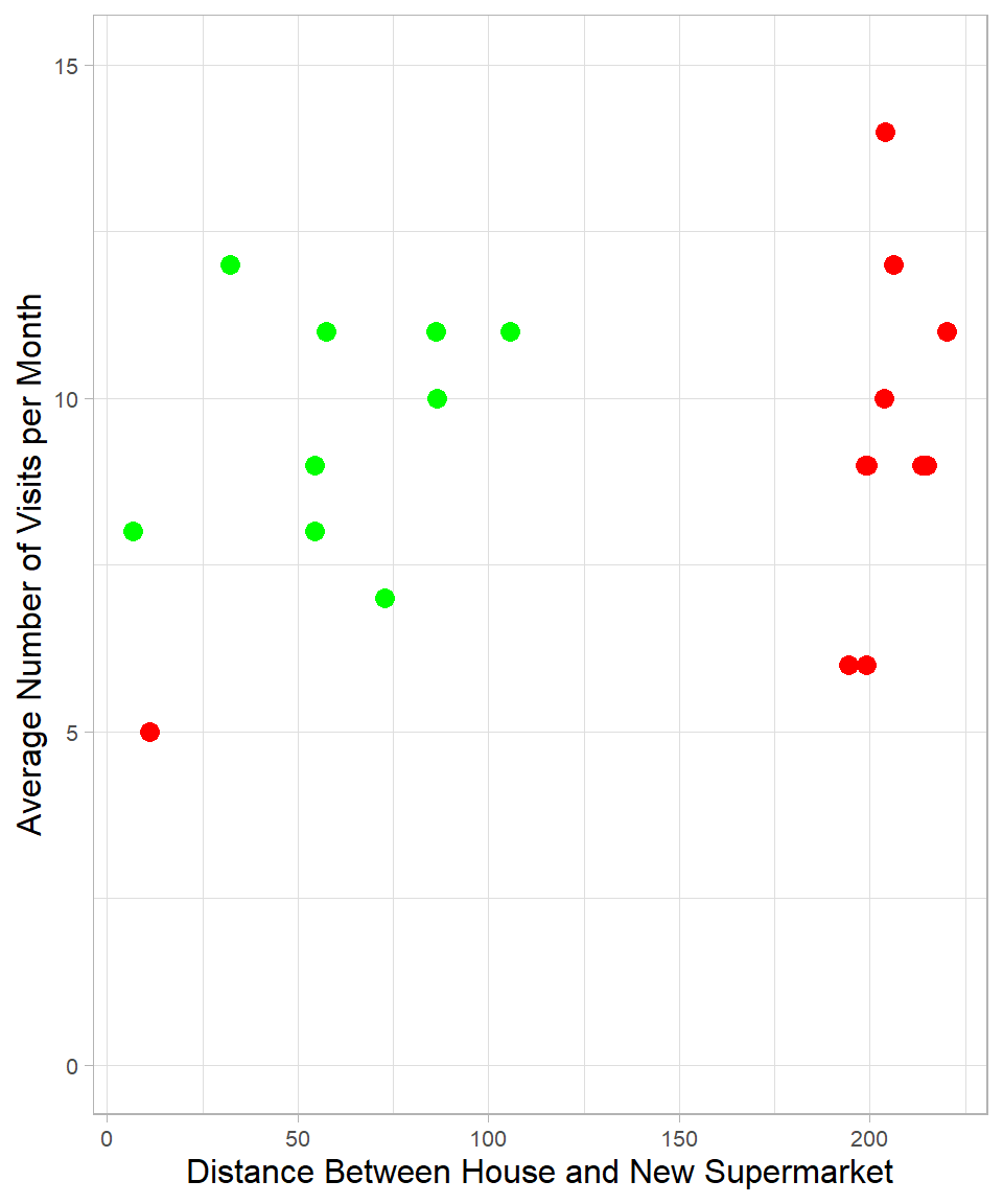
To understand how KNN works, let us return to the supermarket example. Suppose we have two numeric features for each individual: the distance between their house and the new supermarket, and the average number of visits to the new supermarket per month. We collect data on 20 people in your neighborhood. Out of these 20 neighbors, three months after the opening of the new supermarket, 9 decided to start shopping at the new supermarket (green color), while the remaining 11 did not (red color). We can visualize these individuals as points on a two-dimensional plot:
You may notice how the distance from an individual’s house to the new supermarket helps distinguish between the two groups. Almost all the people who visit the new supermarket live closer to it than those who do not. There is one exception: a person who continues shopping at the old supermarket even though the new one is closer. The number of visits per month, on the other hand, seems similar in both groups and does not help as much in making a distinction.
Now suppose your house is located 130 meters from the new supermarket and you visit the supermarket about 10 times per month. We can add your information to the same plot as a new (blue) point:
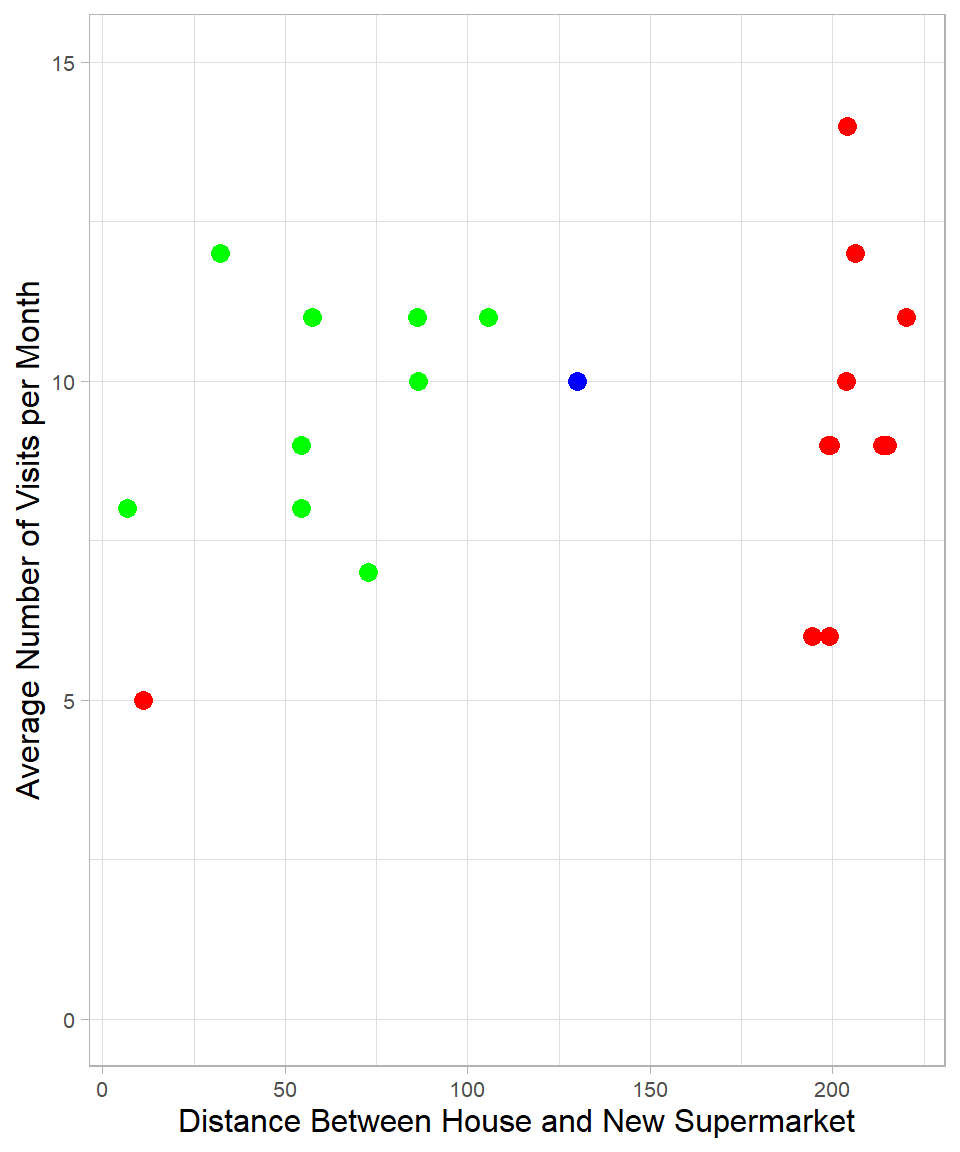
By simply looking at the plot, we might guess that you are more similar to the green group. The nearest neighbor to the blue point is green, so we would classify you as a person who will probably start visiting the new supermarket. This is essentially what the KNN method does. It measures the distance between the blue point and all the other points and assigns a label based on the class of the closest one, or nearest neighbor.
This classification relies on numeric features. An unclassified observation is assigned to the same class as the most similar observations in the training data. Similarity is measured using distances in a multi-dimensional space. In our case, we used two dimensions, but this approach can easily be extended to more.
A natural question arises: how many neighbors should we consider? In other words, how many nearest points should we look at before assigning a class to the new observation? If we use only one neighbor (\(K = 1\)), the blue point would be classified as green. If we consider all 20 neighbors (\(K = 20\)), the majority is red, so the blue point would be classified as red. In case of a tie, the class might be chosen randomly.
Choosing the number of neighbors becomes even more important in more nuanced scenarios. Suppose now your house is only 25 meters from the supermarket, and you visit it 5 times per month. In this case, your closest neighbor is red:
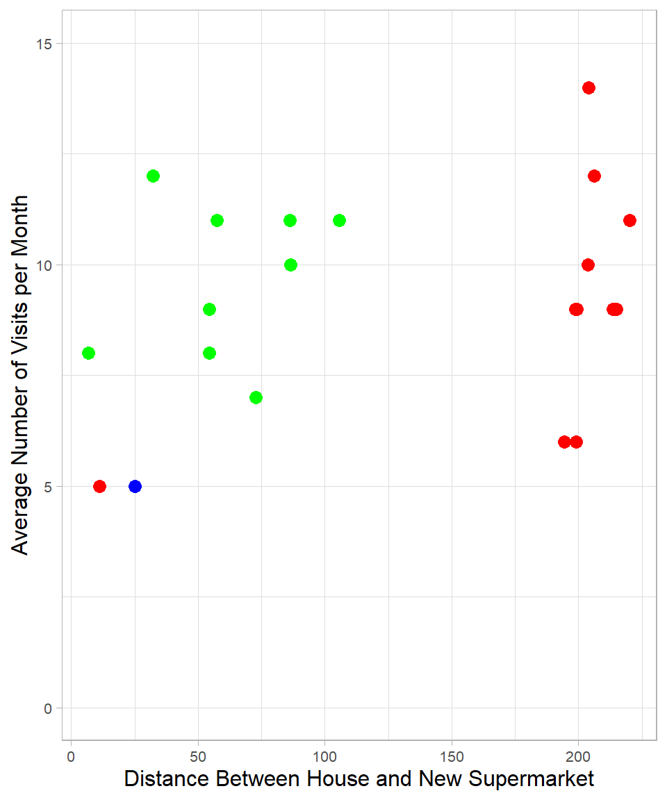
If we choose \(K = 1\), you are classified as red. If we choose \(K = 2\), there is a tie, and the classification could go either way. Choosing higher values of K will increasingly favor green, up until the point where red again becomes the majority due to the higher number of red points overall.
One might argue that the closest neighbor is an exception. However, what if that red neighbor is a close friend and you often shop together? You both visit the supermarket the same number of times per month, which supports this idea. Although we do not have this information in our dataset, it shows that sometimes using only one neighbor might also be reasonable.
\(K\) is actually the main hyperparameter of KNN, a parameter that controls how the model learns (see Chapter Introduction to Machine Learning). There is no universally correct value for \(K\), but a common rule of thumb is to set K equal to the square root of the number of observations in the training set and then try different values to find the most effective one. Generally, a higher \(K\) leads to more consistent results across different samples, while a lower K can make predictions more sensitive to small changes (Lantz, 2023). This reflects the classic bias-variance trade-off, which we discussed in previous chapters.
Measuring the Distance
As explained, to classify a new observation, we need to measure the distance between the point we want to classify and the other points. Although there are different ways to do this, the most commonly used one is the Euclidean distance. To understand how it works, suppose we want to measure the distance between the blue point and the closest green point from Figure 32.1:
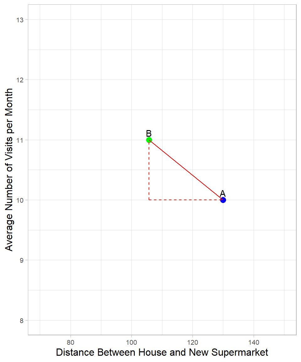
This is the same plot as before, but we focus only on two points. The green and blue points are now labeled B and A respectively. The distance between them is represented by the solid line, and we can apply the Pythagorean Theorem to calculate its length. According to the theorem, the square of the solid line is equal to the sum of the squares of the two dashed lines that form a right triangle. The formula is:
\[\text{dist}(A,B) = \sqrt{(x_{B} - x_{A})^2 + (y_{B} - y_{A})^2}\]
where \(x\) and \(y\) are the variables used to calculate the distance, and \(A\) and \(B\) are the points.
For our example:
\[\text{dist}(A,B) = \sqrt{(x_{B} - x_{A})^2 + (z_{B} - z_{A})^2} = \sqrt{(105 - 130)^2 + (10 - 11)^2} = 25\]
We can extend this formula to more variables, but visualizing it becomes impossible in higher dimensions (at least when more than three dimensions are employed). Still, the underlying logic is the same: we calculate the distance between data points in a multi-dimensional space.
There is, however, an important detail to notice. The formula uses the raw values of the variables, which means that the unit of measurement of each variable can influence the final result. In our case, the distance variable has much larger values than the visit frequency (per month). This causes the distance measure to be driven mostly by the larger-scale variable.
To ensure that each variable contributes equally to the distance calculation, we need to scale our variables. This can be done using min-max scaling or standardization (see Chapter Scaling). Note that the specific values used for scaling depend on the data we have, since the scaling process involves all available data points.
Except for numeric continuous variables, we may also have dummy variables, i.e., variables that take only the values 0 and 1. For instance, a dummy variable might indicate whether a customer used a coupon (1 = Yes, 0 = No). The question is: how do we handle these variables when calculating distances?
Generally, we do not scale dummy variables because they already use a simple and meaningful scale: 0 for “No” and 1 for “Yes”. Scaling typically transforms variables to make them comparable, such as by changing their range (min-max scaling) or converting them into z-scores (standardization). This is important for numeric variables such as the ones we discussed earlier. But for dummy variables, scaling would change the 0s and 1s into values such as -0.3 or 1.7, which blurs their meaning and confuses the algorithm. For example, if we scale the “used a coupon” variable, the values no longer clearly represent a yes-or-no response, making it harder for models such as the KNN to interpret. That’s why we leave dummy variables as they are and only scale the numeric ones when needed.
Apart from dummy variables though, we may have categorical variables with more than two levels. Let’s say we have a variable that shows whether a neighbor owns a motorcycle, a car, both, or no vehicle at all. One way to handle this is to use dummy coding, meaning that we create two dummy variables: one called “Car” and another called “Motorcycle”. If both of these are zero for a neighbor, we know he or she doesn’t have either, meaning that this neighbor belongs to the fourth group: no vehicle. In this way, one category is left out, without losing information. From an algorithmic perspective, it does not matter which category is omitted: the omitted category simply becomes the reference category, and all other categories are interpreted relative to it. The choice only affects the interpretation of the coefficients, not the model’s expressive power or predictive ability.
Another way to use a categorical variable though is with one-hot encoding, which means creating a separate dummy variable for each category, such as “Car”, “Motorcycle”, “Both” and “No Vehicle”. Each neighbor would have a 1 in exactly one of these and 0s in the others. Even though such coding introduces some redundancy, it is easier to understand the output of a model. In the case of KNN, using dummy coding or one-hot encoding does not make a difference in terms of performance.
Assumptions
When we use KNN, we need to keep in mind two specific assumptions, as follows:
Homogeneity: Observations that are close to each other are highly similar (homogeneous) while those that are far away from each other are different. This is actually the main reason that we would choose to apply KNN in the first place: we assume that similar observations belong to the same class (in classification problems) or have the same value of interest (in regression problems).
All features are relevant and equally important: This is also one of the reasons we scale all numeric variables. In case we want one variable to have higher influence on the distance than the others, we need to give more weight to the values of that variable.
By taking the aforementioned assumptions into account, we can assess the suitability of the KNN method for a given problem and make informed decisions during model development and evaluation.
KNN in R
To see how we can use KNN in practice, we use the customer_churn data set, which we have already seen in previous chapters and is available on GitHub. In this example, we use the numeric variables Recency, Frequency, and Monetary_Value to predict whether a customer churns. In other words, our goal is to create a machine learning algorithm (or classifier) that predicts the target (dependent) variable Churn.
# Libraries
library(tidyverse)

# Importing customer_churn
customer_churn <- read_csv("https://raw.githubusercontent.com/DataKortex/Data-Sets/refs/heads/main/customer_churn.csv")
Before we proceed, it is important to clarify what we want as output from our prediction. Because this is a classification problem, the output can take two forms:
- Predicted classes: Here, each observation is assigned a specific class label, either
"Churn"or"Not Churn". This is a “hard” classification where each customer is definitively assigned to one category based on the majority vote among its nearest neighbors. - Estimated probabilities: Instead of a single class, the model can output a probability for each class. These probabilities reflect the proportion of neighbors belonging to each class. For example, if we select 100 neighbors for a given observation and 45 of them have churned, the predicted probability of churn for this observation is 45%. In other words, the probability encodes the level of confidence or likelihood that a customer belongs to a particular class, rather than just giving a binary decision.
In the dataset, the variable Churn takes the value 1 if a customer churned and 0 otherwise. To make class predictions clearer, we create a new variable called Churn_Label, which takes the value "Churn" when Churn == 1 and "No Churn" when Churn == 0. We use Churn_Label for class-based predictions and the original Churn variable for probability-based predictions. Note that Churn_Label must be a factor variable (not a character) for classification.
We use the kknn package to apply the KNN method. Along with kknn, we select only the relevant columns from the dataset, create the Churn_Label variable using the if_else() function, and convert it to a factor:
# Libraries
library(kknn)

# Importing and pre-processing the dataset
customer_churn <- customer_churn %>%
  select(Recency, Frequency, Monetary_Value, Churn) %>%
  mutate(Churn_Label = as.factor(if_else(Churn == 1, "Churn", "No Churn")))
Before we apply standardization, which is generally necessary for KNN, we must first split the data into training and test sets. Standardization must be performed after the split, because using information from the full dataset would leak information from the test set into the training process, leading to overly optimistic performance estimates.
We split the data into 75% training (first 3,000 rows) and 25% test (next 1,000 rows). This is valid here because the rows are already randomly ordered:
# Training and test set split
training_set <- customer_churn %>% slice(1:3000)
test_set <- customer_churn %>% slice(3001:4000)
Now we can apply standardization to the predictors in both data sets:
# Standardization Function
standardization <- function(x) {return((x - mean(x)) / sd(x))}

# Applying standardization on the predictors in the training_set
training_set <- training_set %>%
  mutate(Recency = standardization(Recency),
         Frequency = standardization(Frequency),
         Monetary_Value = standardization(Monetary_Value))

# Applying standardization on the predictors in the test_set
test_set <- test_set %>%
  mutate(Recency = standardization(Recency),
         Frequency = standardization(Frequency),
         Monetary_Value = standardization(Monetary_Value))
With preprocessing complete, we now build the KNN classifier using the function kknn(). As with other modeling functions such as lm(), the formula format is:
\[ y \sim x \]
where \(y\) is the target variable and \(x\) includes all predictors.
Let’s create a KNN classifier using k = 2, with Churn_Label as the target variable:
# KNN Classifier with k equal to 2
knn_classifier <- kknn(Churn_Label ~ Recency + Frequency + Monetary_Value,
                       train = training_set,
                       test = test_set,
                       k = 2)
The knn_classifier object contains several components, including the predicted values for the observations in the test set. These predictions are stored in the $fitted.values element of the object. Therefore, knn_classifier$fitted.values provides the predicted class labels for each observation in the test set, based on the \(K\) nearest neighbors from the training set:
# Printing the first 6 predictions
knn_classifier$fitted.values %>% head(n = 6)
[1] No Churn No Churn No Churn No Churn No Churn No Churn
Levels: Churn No ChurnJust like in regression problems, there are different metrics to assess classification accuracy. For classification, the simplest metric is accuracy, which measures the proportion of correct predictions:
\[\text{Accuracy} = \frac{\text{Number of correct predictions}}{\text{Number of observations}}\]
Essentially, accuracy is just the average of these 0–1 indicators across all observations, which is why we can compute it in R using the mean() function:
# Calculating accuracy
mean(knn_classifier$fitted.values == test_set$Churn_Label)
[1] 0.815This gives the overall accuracy of the classifier on the test set.
A natural follow-up question is: what would the accuracy be if we always predicted the majority class? Since most customers do not churn, always predicting “No Churn” should yield an accuracy above 50%. This baseline is known as the No Information Rate (NIR):
# Calculating NIF
mean("No Churn" == test_set$Churn_Label)
[1] 0.742In our case, the KNN model achieves an accuracy above 80%, while the NIR is below 75%, showing that the model provides meaningful predictive improvement over a naive baseline.
Now, let’s set k = 5 and re-evaluate accuracy:
# KNN Classifier with k equal to 5
knn_classifier <- kknn(Churn_Label ~ Recency + Frequency + Monetary_Value,
                       train = training_set,
                       test = test_set,
                       k = 5)

# Calculating accuracy
mean(knn_classifier$fitted.values == test_set$Churn_Label)
[1] 0.863Accuracy improves further, indicating that k = 2 was not optimal. This illustrates that model performance depends not only on the predictors, but also on hyperparameters such as \(K\).
If we use the numeric variable Churn instead of the factor variable Churn_Label, the predicted values from the model represent the estimated probability that each customer will churn:
# KNN Classifier with k equal to 2
knn_classifier <- kknn(Churn ~ Recency + Frequency + Monetary_Value,
                       train = training_set,
                       test = test_set,
                       k = 2)

# Printing the first 6 fitted values
knn_classifier$fitted.values %>% head(n = 6)
[1] 0.0000000 0.0000000 0.2224704 0.0000000 0.0000000 0.0000000The predicted values now lie between 0 and 1, where higher values indicate higher churn risk.
To evaluate performance, we convert probabilities into class predictions using a threshold. With a 50% threshold, customers with predicted probability of at least 50% are classified as churners:
# Predicted classes based on the estimated probabilities
p <- if_else(knn_classifier$fitted.values >= 0.5, "Churn", "Not Churn")

# Performance of the classifier
mean(p == test_set$Churn_Label)
[1] 0.167Notice that the accuracy is exactly the same as before. This is because a 50% threshold mimics the decision rule used when Churn_Label is the target. In other words, 50% is the default threshold when we use a dependent variable that is a factor with two levels.
However, using probabilities instead of hard class predictions can be more useful in practice. For instance, both a customer with 51% and a customer with 95% churn probability would be classified as churners, but the risk level is not the same. A business might use different thresholds, such as 45%, to classify more customers as potential churners and intervene earlier.
Although we focused on classification problems, KNN can also be used for regression, where the dependent variable is continuous. In such cases, the predicted value for an observation is the average of the dependent variable values of its nearest neighbors. The same logic and the same kknn() function can be used.
Advantages and Limitations
KNN is a simple and intuitive method, which makes it particularly appealing for practical applications. It requires no explicit model training, as predictions are made by comparing new observations to the training data in real time (Lantz, 2023). This flexibility allows KNN to handle both classification and regression tasks, and its performance does not rely on any specific assumptions about the underlying data distribution. These properties make KNN especially useful for datasets with complex or unknown patterns, or when the relationships between features and the target variable are not easily captured by parametric models such as linear regression.
Despite its simplicity, KNN has some notable limitations. Because it compares each new observation to all points in the training set, it can become computationally expensive for large datasets (Taunk, De, & Verma, 2019). The method is also highly sensitive to feature scaling and irrelevant features, which links back to the key assumption that all features are relevant and equally important. Choosing the number of neighbors, K, is another critical step: too small a value can lead to overfitting, while too large a value may smooth over meaningful patterns and reduce predictive accuracy. Finally, KNN can struggle with high-dimensional data due to the curse of dimensionality, especially compared to many other machine learning methods. As the number of features increases, the concept of “distance” becomes less informative, which can undermine performance.
When applied to datasets with a modest number of well-scaled and relevant features, KNN can be highly effective, providing strong predictive performance in tasks ranging from customer churn prediction to anomaly detection and recommendation systems.
Recap
K-Nearest Neighbors (KNN) is a simple and intuitive method for both classification and regression tasks. It makes predictions by comparing a new observation to its nearest neighbors in the training data, using a distance metric such as Euclidean distance. The main hyperparameter \(K\) determines how many neighbors influence the prediction, balancing sensitivity to individual points and overall stability. KNN assumes that similar observations are close in feature space and that all features contribute equally to defining similarity, which is why feature scaling is essential.
While KNN requires no explicit model training and adapts naturally to complex patterns, it can be computationally expensive for large datasets and is sensitive to irrelevant or poorly scaled features. It also struggles in high-dimensional spaces, where distance becomes less informative. Despite these limitations, KNN can deliver accurate and interpretable predictions, as seen in examples such as customer churn classification.