In linear regression, knowing the expected value and variance of an estimated coefficient is essential for understanding the key properties of unbiasedness and efficiency. However, knowing the expected value and the variance of a sampling distribution of an estimated coefficient, does not say anything about the form of the distribution; it could be normal uniform or even poisson.
This means that the expected value and variance are not sufficient alone for making statistical inference—that is, drawing conclusions about the population from the sample data. As we discussed in the chapter Hypothesis Testing, statistical inference relies on theoretical probability distributions to quantify uncertainty and evaluate the likelihood of various hypotheses.
The distribution we use for inference depends on the context. It could be a normal distribution, a t-distribution, or something else entirely, such as the uniform distribution we encountered earlier. In the case of linear regression, statistical inference typically builds on the sampling distribution of the estimated coefficients, which—under certain assumptions—follows a t-distribution.
In this chapter, we explore how linear regression can be used not only to estimate relationships but also to conduct formal inference. We build on the concepts developed in earlier chapters, including sampling distributions, standard errors, hypothesis testing, and confidence intervals. In that sense, there is nothing entirely new here—rather, we bring together several familiar ideas and apply them in the context of regression. Our focus will be on how to test whether a coefficient is significantly different from zero and how to construct confidence intervals for the estimated coefficients.
We also introduce a few helpful R functions that make these tasks straightforward in practice. This chapter is where theory meets application: we now use regression not just as a modeling tool, but also as a framework for reasoning under uncertainty.
From Estimation to Hypothesis Testing
Let us now return to the multiple linear regression model. We begin by loading the tidyverse package, importing the dataset from GitHub, and regressing Revenue on Ad_Spend, Product_Quality_Score, and Website_Visitors:
# Librarieslibrary(tidyverse)# Importing eshop_revenueseshop_revenues <-read_csv("https://raw.githubusercontent.com/DataKortex/Data-Sets/refs/heads/main/eshop_revenues.csv")# Fitting a linear regression modellm_model <-lm(Revenue ~ Ad_Spend + Product_Quality_Score + Website_Visitors, data = eshop_revenues)# Printing coefficientsprint(lm_model)
Now that we have the coefficient estimates, we are equipped to interpret the expected change in revenue associated with each independent variable. But an important question remains: are these effects statistically significant? For example, if the coefficient on Website_Visitors is 0.001, it implies that, holding other variables constant, revenue is expected to increase by only €1 for every 1,000 additional visitors. This effect may be negligible in practice. We need statistical inference to determine whether such an effect is distinguishable from zero in the pop
As discussed in Chapter Hypothesis Testing, we must formulate a null hypothesis and an alternative hypothesis to guide our inference. In regression analysis, we typically test whether each coefficient is significantly different from zero. For example, the hypotheses for the coefficient on Ad_Spend might be:
\(H_0: \beta_1 = 0\)
\(H_1: \beta_1 \ne 0\)
To evaluate these hypotheses, we conduct a one sample t-test for each coefficient. The formula for the t-statistic is:
Here, \(\hat{\beta}_{i}\) is the estimated coefficient, \(\beta_{i}\) is the hypothesized value under the null (typically 0), and \(SE(\hat{\beta}_{i})\) is the standard error of the estimate. As we saw in earlier chapters, the standard error is derived from the residual variance of the model and reflects how much the estimate would vary across repeated samples.
Once we have the t-value, we compare it to the t-distribution with the appropriate degrees of freedom to determine whether the observed value is extreme enough to reject the null hypothesis. Everything else we learnt about hypothesis testing such as critical value, p-value, confidence interval, etc. applies here.
The coefficients, standard errors, t-values, and their corresponding p-values are all automatically computed when we use the lm() function in R. To access and display them, we use the summary() function on the model object. This summary provides a complete overview of the estimated coefficients, their variability across samples, the results of the hypothesis tests (via the t-values), and the associated p-values that indicate whether each coefficient is statistically significant.
Call:
lm(formula = Revenue ~ Ad_Spend + Product_Quality_Score + Website_Visitors,
    data = eshop_revenues)

Residuals:
   Min     1Q Median     3Q    Max
-37767  -6250   -745   3936  46169

Coefficients:
                        Estimate Std. Error t value Pr(>|t|)
(Intercept)           -35222.037   5749.350  -6.126 1.06e-08 ***
Ad_Spend                  48.888      5.914   8.267 1.64e-13 ***
Product_Quality_Score   5030.115    784.281   6.414 2.60e-09 ***
Website_Visitors           7.791      3.944   1.975   0.0504 .
---
Signif. codes:  0 '***' 0.001 '**' 0.01 '*' 0.05 '.' 0.1 ' ' 1

Residual standard error: 10510 on 126 degrees of freedom
Multiple R-squared:  0.5849,    Adjusted R-squared:  0.575
F-statistic: 59.17 on 3 and 126 DF,  p-value: < 2.2e-16
This output contains several important elements that allow us to perform statistical inference.
Let us walk through the key parts:
Call: The first line simply displays the formula used to specify the model. This helps verify that we regressed the correct dependent variable on the appropriate predictors.
Residuals: This section summarizes the distribution of the residuals—i.e., the differences between the observed and predicted values of the dependent variable. It reports five summary statistics: the minimum, 1st quartile, median, 3rd quartile, and maximum. Ideally, the residuals should be symmetrically distributed around zero, which would support the assumption of zero-mean errors.
Coefficients: This is the core table for inference. Each row corresponds to a model parameter (intercept or slope), and each column provides important information.
Estimate: The estimated value of the coefficient \(\hat{\beta}_{i}\).
Std. Error: The standard error of the estimate, reflecting its variability across repeated samples.
used to evaluate the null hypothesis that \(\beta_{i} = 0\).
Pr(>|t|): The p-value associated with the t-test. A small p-value (typically below 0.05) provides evidence against the null hypothesis, suggesting that the coefficient is statistically significant.
The table may also include symbols such as * or ** to indicate significance levels, often based on conventional thresholds (e.g., 0.1, 0.05, 0.01). These visual cues help quickly identify which predictors are statistically significant.
Residual standard error: This is an estimate of the standard deviation ( \(\sqrt{\sigma^2}\) )of the residuals.
Degrees of freedom: This tells us how many observations and predictors were used, which determines the shape of the t-distribution used in the hypothesis tests.
R-squared and Adjusted R-squared: These values summarize how well the model explains the variability in the dependent variable. R-squared gives the proportion of variance explained by the model, while the adjusted version accounts for the number of predictors, penalizing unnecessary complexity.
We will return to the last line of the output regarding the F-statistic and its p-value later in this chapter, when we discuss how to evaluate the overall significance of a regression model.
Regarding our example output, the p-values for almost all coefficients are statistically significant at the 5% significance level, indicating that these predictors have meaningful associations with the dependent variable. One borderline case is the coefficient for Website_Visitors, which has a p-value of 0.0504 which slightly above the conventional 5% threshold. While this technically does not meet the cutoff for significance, it is extremely close, and such small differences are often considered with caution and interpreted in context rather than rigidly.
The R-squared and Adjusted R-squared values are 58.49% and 57.50%, respectively. The fact that these two values are close suggests that the model does not include unnecessary predictors. The Adjusted R-squared penalizes the inclusion of additional variables that do not improve the model, so when it remains close to the R-squared, it provides reassurance that each variable contributes meaningfully to explaining the variation in the dependent variable.
Assumptions
As stated earlier, knowing the expected value and variance of an estimated coefficient is helpful for understanding unbiasedness and efficiency. However, it is not sufficient for making statistical inference. To conduct hypothesis tests, such as the t-test, we rely on theoretical distributions. This introduces one additional assumption required for inference in the classical linear regression model: the normality assumption.
The assumption of normality states that the error terms in the regression model are normally distributed with a mean of zero and constant variance. Mathematically, this is written as:
\[u \sim N(0, \sigma^2)\]
We have already assumed that the error terms have an expected value of zero (i.e., they are centered around zero), and that they all share the same constant variance, \(\sigma^2\). The normality assumption adds that the shape of the distribution is also known: it is bell-shaped, symmetric, and follows the normal (Gaussian) distribution.
This assumption carries over to the distribution of the dependent variable \(y\) conditional on the values of the independent variables \(\mathbf{X}\). In other words:
This means that for any fixed point in the multidimensional space of the independent variables, the value of \(y\) is normally distributed around its conditional mean. That is, holding the independent variables fixed, \(y\) behaves like a normal random variable.
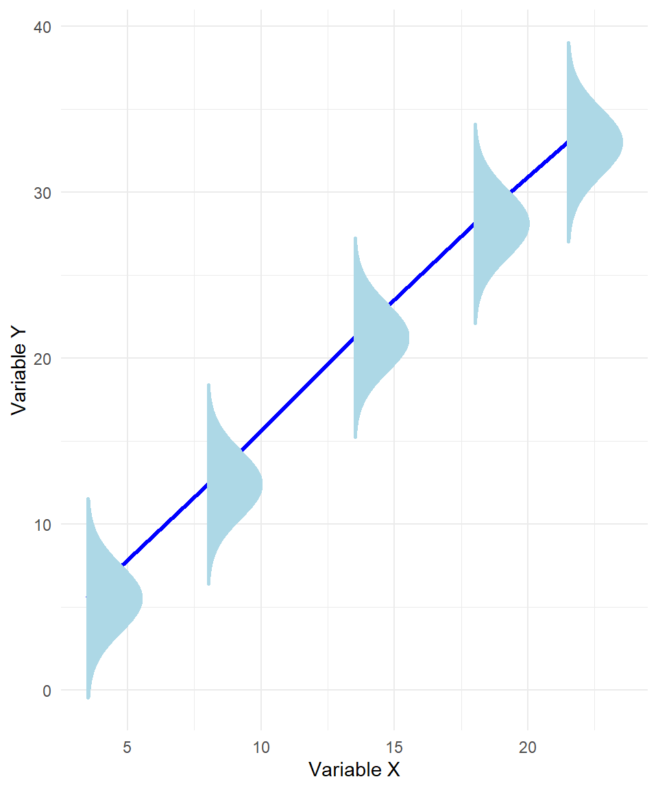
The plot below illustrates a key assumption of linear regression: that the response variable \(y\) follows a normal distribution around the regression line at every value of \(x\). At several points along the line, we’ve visualized this by drawing normal distribution “tunnels”, each centered at the predicted value of \(y\) for a given \(x\). This highlights the normality assumption of the errors—that the variability in \(y\) at each level of \(x\) is random and normally distributed. If this assumption holds, and the relationship between \(x\) and \(y\) is truly linear, then the red regression line represents the best possible linear estimate of the expected value of \(y\) given \(x\). In other words, under these conditions, there is no better straight line we could draw to capture the average behavior of \(y\) across values of \(x\).
Figure 25.1: Linear regression line when normality holds.
Because the OLS estimates are linear combinations of the dependent variable \(y\), and \(y\) is normally distributed, it follows that the estimated coefficients themselves are also normally distributed:
More generally, any linear combination of the estimated coefficients, such as \(c_1 \hat{\beta}_1 + c_2 \hat{\beta}_2\), is also normally distributed. This property allows us to construct confidence intervals and conduct hypothesis tests on individual coefficients as well as combinations of them.
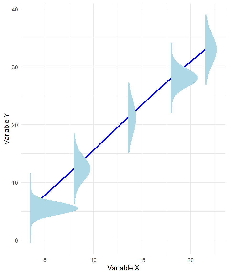
An example of where normality would not hold can be viewed in the plot below:
Figure 25.2: Linear regression line when normality does not hold.
Even though linear regression still seems to be the best fit, Even though the regression line fits the data, the spread of the points around the line is not the same everywhere—some points are very close to the line, while others are much more spread out. If we ask, “Is the estimated slope statistically significantly different from 0?”, the answer can depend on which part of the x-axis we are looking at. In other words, we are no longer fully confident about whether the estimated slope of the regression line is truly different from 0.
Thus, to assume normality of the OLS estimates, we must also assume the five classical conditions discussed in earlier chapters:
Linearity in parameters
Random sampling
Sample variation and no perfect multicollinearity
Zero conditional mean of errors
Homoskedasticity (constant error variance)
By adding normality of the error terms, we now have a sixth assumption. Together, these six assumptions define what is known as the Classical Linear Model (CLM). Under these assumptions, OLS estimators are not only BLUE (Best Linear Unbiased Estimators, as stated by the Gauss-Markov theorem), but also normally distributed, allowing us to perform valid statistical inference using t- and F-tests (Wooldridge, 2022).
Surpringly, even if the normality assumption is violated, statistical inference may still be valid when the sample size is sufficiently large. This is due to the Central Limit Theorem (CLT). The CLT states that, under certain regularity conditions, the distribution of the sample mean (and more generally, linear estimators such as OLS) approaches a normal distribution as the sample size increases. This means that, in large samples, the estimated coefficients will still be approximately normally distributed, even if the original error terms are not. As a result, t-tests and confidence intervals based on the normal distribution become asymptotically valid (Wooldridge, 2022).
The term asymptotically refers to what happens as the sample size tends toward infinity. In other words, asymptotic properties describe the behavior of estimators when we imagine having more and more data. An estimator is said to be asymptotically normal if its distribution becomes closer to the normal distribution as the sample size increases. Similarly, a test is asymptotically valid if its conclusions (e.g., rejecting or not rejecting the null hypothesis) become increasingly accurate and reliable with more data.
It is important to note that asymptotic results are not exact in finite samples. They are approximations that improve with larger sample sizes. Therefore, in small datasets, we still prefer to assume normality explicitly if we want to use t-tests or construct confidence intervals.
The concept of asymptotic validity may not seem practical and in fact it isn’t; it is primarily theoretical. It helps us understand the long-run behavior of estimators and statistical tests under general conditions. In practice, we never observe an infinite sample—so these results guide our expectations and justify the use of certain methods in large samples, rather than serving as a guarantee in every case.
The bottom line is that normality is crucial for making exact inferences in small samples. It allows us to use the t-distribution to construct confidence intervals and perform hypothesis testing on regression coefficients. However, in large samples, even if the error terms are not perfectly normal, the Central Limit Theorem helps ensure that our estimates and statistical tests remain approximately valid. In this way, normality is a helpful but not always essential assumption—its importance depends on the sample size.
F-test in Linear Regression
In Chapter Chi-Square and F-Distributions, we discussed how the F-test can be used to compare two variances and determine whether they are significantly different. In the context of linear regression, the F-test serves a related purpose: it evaluates whether the model as a whole provides a significantly better fit to the data than a model with no predictors at all.
Recall that the goal of regression is to explain the variation in the dependent variable \(y\) using the independent variables. When we run a regression, we effectively decompose the total variation in \(y\)—the Total Sum of Squares (TSS)—into two parts:
The part explained by the regression: Explained Sum of Squares (ESS)
The part not explained: the Residual Sum of Squares (RSS).
Mathematically:
\[\text{TSS} = \text{ESS} + \text{RSS}\]
The RSS captures the unexplained variance—the differences between the observed values and the values predicted by our model. If the model has little explanatory power, the RSS will be large compared to the TSS. If the model explains a significant portion of the variance, the RSS will be relatively small, and the ESS will be large.
The F-statistic is a ratio that compares the amount of variance explained by the model to the amount left unexplained, adjusted for the number of predictors and the number of observations. It is calculated as:
\(k\) is the number of predictors (excluding the intercept),
\(n\) is the number of observations.
This formula compares the explained variance per predictor to the unexplained variance per residual degree of freedom. A high F-value suggests that the model explains a significant portion of the variance in \(y\), relative to what remains unexplained.
We can manually calculate the F-statistic in R using the following code:
# Actual valuesy <- eshop_revenues$Revenue# Predicted valuesy_hat <- lm_model$fitted.values# Mean of yy_bar <-mean(y)# Total Sum of SquaresTSS <-sum((y - y_bar)^2)# Residual Sum of SquaresRSS <-sum((y - y_hat)^2)# Number of predictorsk <-3# Sample sizen <-130# F-statistic formulaF_stat <- ((TSS - RSS) / k) / (RSS / (n - k -1))# Printing F-statisticF_stat
[1] 59.16957
This gives us the same F-statistic as the one printed at the bottom of the regression output when using the summary() function:
Call:
lm(formula = Revenue ~ Ad_Spend + Product_Quality_Score + Website_Visitors,
    data = eshop_revenues)

Residuals:
   Min     1Q Median     3Q    Max
-37767  -6250   -745   3936  46169

Coefficients:
                        Estimate Std. Error t value Pr(>|t|)
(Intercept)           -35222.037   5749.350  -6.126 1.06e-08 ***
Ad_Spend                  48.888      5.914   8.267 1.64e-13 ***
Product_Quality_Score   5030.115    784.281   6.414 2.60e-09 ***
Website_Visitors           7.791      3.944   1.975   0.0504 .
---
Signif. codes:  0 '***' 0.001 '**' 0.01 '*' 0.05 '.' 0.1 ' ' 1

Residual standard error: 10510 on 126 degrees of freedom
Multiple R-squared:  0.5849,    Adjusted R-squared:  0.575
F-statistic: 59.17 on 3 and 126 DF,  p-value: < 2.2e-16
The degrees of freedom (3 and 126) in the F-test output correspond to the number of predictors (\(k = 3\)) and the residual degrees of freedom (\(n − k − 1 = 126\)), respectively. The associated p-value is derived from the F-distribution with these degrees of freedom.
From a hypothesis testing perspective, the F-test evaluates the null hypothesis that all regression coefficients are equal to zero:
against the alternative hypothesis that at least one coefficient is non-zero.
This test does not include the intercept, because we always estimate it by default. It is called the F-test of overall significance, because it checks whether the model, as a whole, explains a statistically significant portion of the variation in the dependent variable.
We can also express the F-statistic in terms of the \(R^2\) value:
\[F = \frac{R^2 / k}{(1 - R^2) / (n - k - 1)}\]
This version shows that as \(R^2\) increases, meaning a better model fit, the F-statistic becomes larger, increasing the chance of rejecting the null hypothesis. In other words, a high F-statistic implies that the model explains a meaningful amount of variation in \(y\), suggesting that at least one of the predictors is statistically significant.
The F-test, however, can be used for more than just testing the overall significance of a regression model. It is also a powerful tool for comparing different linear regression models, especially when one model is a special case (or a subset) of another. This situation arises when one model includes fewer predictors than the other.
For instance, consider the following two regression models:
Here, the first model is a simplified version of the second—it includes only one predictor (AdSpend) instead of three. Because of this, it’s called the restricted model, while the second, more flexible model is the unrestricted model.
The unrestricted model adds ProductQualityScore and WebsiteVisitors. The F-test allows us to check whether these two additional variables jointly improve the model. In other words, we test whether their coefficients (𝛽₂ and 𝛽₃) are both equal to zero.
Both models explain a portion of the total variance in Revenue. The F-test compares how much the residual sum of squares (RSS) decreases when moving from the restricted to the unrestricted model. If the drop is large enough relative to the added complexity, the improvement is considered statistically significant. This joint testing is useful because even if individual t-tests for 𝛽₂ and 𝛽₃ are not significant, the F-test might still show that the variables are jointly significant.
\(\text{RSS}_{R}\): Residual sum of squares of the restricted model
\(\text{RSS}_{UR}\): Residual sum of squares of the unrestricted model
\(q\): Number of restrictions (i.e., the number of additional variables tested jointly)
\(k\): Number of predictors in the unrestricted model
\(n\): Sample size
This is also known as a joint hypothesis test, because it tests multiple coefficients at once. If the resulting p-value is below the chosen significance level (e.g., 0.05), we conclude that the additional variables are jointly statistically significant, meaning they contribute meaningfully to the model. Otherwise, they are jointly statistically insignificant.
Why Joint Significance
You might wonder: Why not just check the individual t-values of the added variables in the unrestricted model? The answer is that individual t-tests assess each coefficient one at a time, while holding all others fixed. But when predictors are correlated, t-tests can fail to detect joint effects. It’s actually quite common that none of the individual t-tests shows significance, yet the variables are jointly significant when tested together. This is especially important when we are adding a set of related variables. In such cases, the F-test provides a more comprehensive view of whether the group of variables, as a whole, improves the model.
Tidy Model Summaries and Hypothesis Testing in R
As previously discussed, when we fit a linear model using lm(), R automatically computes a variety of useful statistics. To extract this information, we can use the dollar ($) sign, the summary() function or even other functions that are easily applicable such as coef() or residuals().
However, there’s a more structured and efficient way to extract and organize model results. The broom package, created by Dave Robinson, offers a convenient and tidy way to extract and work with model outputs. It includes three key functions:
tidy(): This function extracts coefficient-level statistics, such as estimates, standard errors, t-values, and p-values, and returns them as a clean data frame. This makes it easier to view, manipulate, and visualize regression results. We can also include confidence intervals for the coefficients, you can simply set conf.int = TRUE and specify the desired confidence level using the conf.level argument.
# Librarieslibrary(broom)# Applying the tidy() functiontidy(lm_model, conf.int =TRUE, conf.level =0.95)
augment(): This function adds information to the original dataset, such as fitted values (.fitted), residuals (.resid), and leverage. It essentially combines the raw data with model diagnostics, allowing for quick exploration of how well the model fits each observation.
# Applying the augment() functionaugment(lm_model, data = eshop_revenues)
glance(): This function returns a one-row summary of model-level statistics such as R-squared, adjusted R-squared, sigma and F-statistic, and other metrics we have not discussed such as AIC and BIC. It’s useful when comparing multiple models or summarizing fit statistics at a glance. At this point
While the t-tests from lm() (or tidy()) check one coefficient at a time, we often want to test multiple coefficients simultaneously. This is where the linearHypothesis() function from the car package becomes useful. It allows us to perform joint hypothesis testing or test more general linear restrictions on the coefficients. The function requires the model object (typically created by lm()) and a character string (or vector of strings) specifying the hypotheses, using the exact variable names as they appear in the model.
For example, suppose we want to test whether the coefficient of Ad_Spend is equal to 50:
Linear hypothesis test:
Product_Quality_Score = 0
Website_Visitors = 0

Model 1: restricted model
Model 2: Revenue ~ Ad_Spend + Product_Quality_Score + Website_Visitors

  Res.Df        RSS Df  Sum of Sq      F    Pr(>F)
1    128 2.0023e+10
2    126 1.3925e+10  2 6098082321 27.589 1.155e-10 ***
---
Signif. codes:  0 '***' 0.001 '**' 0.01 '*' 0.05 '.' 0.1 ' ' 1
This produces an F-statistic and p-value for the joint hypothesis that both coefficients are zero. This is particularly useful when evaluating whether a group of predictors adds significant explanatory power to the model.
In fact, if we use linearHypothesis() to test whether all coefficients (except the intercept) are equal to zero, we are effectively reproducing the F-test for overall significance that appears at the bottom of the output from summary(lm_model).
Linear hypothesis test:
Ad_Spend = 0
Product_Quality_Score = 0
Website_Visitors = 0

Model 1: restricted model
Model 2: Revenue ~ Ad_Spend + Product_Quality_Score + Website_Visitors

  Res.Df        RSS Df  Sum of Sq     F    Pr(>F)
1    129 3.3542e+10
2    126 1.3925e+10  3 1.9617e+10 59.17 < 2.2e-16 ***
---
Signif. codes:  0 '***' 0.001 '**' 0.01 '*' 0.05 '.' 0.1 ' ' 1
The resulting F-statistic is 59.17, the same we got earlier by using the summary() function.
Heteroskedasticity
Up to this point, we have discussed the assumptions necessary for obtaining BLUE (Best Linear Unbiased Estimator) estimates, one of which is homoskedasticity—the assumption that the variance of the errors remains constant across all values of the independent variables. If this assumption is violated, we have heteroskedasticity, which means the Gauss–Markov theorem no longer applies, and the OLS estimates, while still unbiased, are no longer efficient (Wooldridge, 2022).
When working with just one or even two independent variables, detecting heteroskedasticity is often feasible using visual tools. However, when the model involves multiple predictors, visual inspection becomes more challenging, and formal statistical tests become more useful.
One commonly used test is the F-version of the Breusch–Pagan test. The logic behind this test is straightforward. If the homoskedasticity assumption holds, then the variance of the error terms should not systematically vary with the values of the independent variables. In other words, there should be no association between the independent variables and the squared residuals from the model.
Mathematically, homoskedasticity implies that the variance of the error terms is constant across all observations, often written as \(Var(u_i) = \sigma^2\) for all \(i\). When this assumption is violated, the variance is no longer constant but varies with each observation. In that case, we write \(Var(u_i) = \sigma^2_i\), indicating that each error term has its own variance. This heterogeneity in the error variances is precisely what the Breusch–Pagan test is designed to detect.
To test whether the homoskedasticity assumption holds, we first obtain the residuals from the original regression model and square them. Then, we run a new regression where the squared residuals serve as the dependent variable and the original independent variables remain as predictors. If homoskedasticity holds, none of the predictors should significantly explain the variation in the squared residuals, and the F-statistic from this additional regression should be low, resulting in a high p-value. This would lead us to fail to reject the null hypothesis, which is the hypothesis of homoskedasticity.
Here is how we can implement this in R:
# Extracting residuals and square themu <- lm_model %>%residuals()u_squared <- u^2# Auxiliary regression: squared residuals on original predictorslm(u_squared ~ Ad_Spend + Product_Quality_Score + Website_Visitors, data = eshop_revenues) %>%summary()
Call:
lm(formula = u_squared ~ Ad_Spend + Product_Quality_Score + Website_Visitors,
    data = eshop_revenues)

Residuals:
       Min         1Q     Median         3Q        Max
-655800004  -92496960   -6464980   43662514 1669907169

Coefficients:
                        Estimate Std. Error t value Pr(>|t|)
(Intercept)           -198233593  118194894  -1.677    0.096 .
Ad_Spend                  873170     121577   7.182 5.28e-11 ***
Product_Quality_Score    4125727   16123211   0.256    0.798
Website_Visitors           98372      81089   1.213    0.227
---
Signif. codes:  0 '***' 0.001 '**' 0.01 '*' 0.05 '.' 0.1 ' ' 1

Residual standard error: 216100000 on 126 degrees of freedom
Multiple R-squared:  0.3834,    Adjusted R-squared:  0.3687
F-statistic: 26.12 on 3 and 126 DF,  p-value: 3.317e-13
In this output, we are primarily interested in the p-value of the F-statistic, which tests the joint significance of the independent variables in explaining the squared residuals. If this p-value is small (e.g. below 0.05 or 0.01), we reject the null hypothesis of constant variance, indicating that heteroskedasticity is present.
In the example above, the p-value of the F-statistic is very low, even at the 1% significance level. This suggests strong evidence of heteroskedasticity. Additionally, we can examine the individual coefficients in the auxiliary regression. If one or more variables (e.g., Ad_Spend) are statistically significant, they may be contributing more heavily to the unequal variance of residuals. This can provide useful diagnostic insight, though the F-test result remains the primary evidence of heteroskedasticity.
In summary, the Breusch–Pagan test offers a formal and interpretable method for testing the homoskedasticity assumption, which is crucial for the validity of standard errors, confidence intervals, and hypothesis tests in linear regression models.
Using External Vectors in lm()
In the last code chunk, we were able to use the vector u_squared in the regression formula even though it is not a column in the data frame dat. This works in R because when we run a regression using the lm() function, R first evaluates the objects in the global environment. Since u_squared exists as a separate vector in memory (and has the same length as the rows in dat), R is able to align it correctly with the corresponding observations. It is important to remember that this only works if the vector is the same length as the number of observations in the data frame and is in the same order. An alternative approach would be to save the squared residuals in a separate column in the dat object and then use the lm() function.
Breusch-Pagan Test: LM vs. F Versions
Earlier, we introduced the Breusch-Pagan F-test to detect heteroskedasticity. To be precise, this is one version of the Breusch-Pagan test—specifically, the F-version. There is also a Lagrange Multiplier (LM) version, which differs mainly in the distribution used for the test statistic: the F-version uses an F-distribution, while the LM version uses a chi-square distribution.
Both versions work in the same way: they regress the squared residuals on the independent variables to check whether the error variance depends on them. In practice, the LM version is more common for larger samples, whereas the F-version can be easier to interpret with smaller samples. A significant result in either test indicates heteroskedasticity, meaning that the OLS assumptions are violated and coefficient estimates may be inefficient.
For most datasets, both versions lead to the same conclusion, with differences appearing mainly in very small samples or unusual data. Therefore, whether you use the F-version or the LM (chi-square) version, the inference about heteroskedasticity is typically the same.
If we detect heteroskedasticity, we know that our inference can be incorrect and that the ordinary least squares (OLS) estimated coefficients are no longer BLUE (Best Linear Unbiased Estimators). While alternative estimation methods exist, a more common and practical approach is to adjust the standard errors to account for heteroskedasticity.
Heteroskedasticity implies that the variance of the error terms changes with the values of the independent variables, violating the assumption of constant variance. Because of this, the usual formula for calculating the variance of the coefficient estimates is no longer valid. Instead, we use robust standard errors, which provide consistent estimates of the coefficient variances even when heteroskedasticity is present.
These heteroskedasticity-robust standard errors allow us to perform valid hypothesis tests and construct reliable confidence intervals without changing the estimated coefficients themselves. This adjustment is widely used in applied regression analysis because it is easy to implement and does not require changing the model.
In R, we can easily compute heteroskedasticity-robust standard errors using the packages sandwich and lmtest. These packages work together to provide a flexible and convenient way to correct for heteroskedasticity in linear models.
vcovHC() from the sandwich package calculates a heteroskedasticity-consistent (robust) variance-covariance matrix for the coefficients of a linear model. The argument type = "HC1" specifies the version of the robust estimator. Even though there are other types such as "HC0", "HC2", or "HC3", each with slightly different adjustments, "HC1" is commonly used in practice.
coeftest() from the lmtest package performs hypothesis tests (e.g., t-tests) on the coefficients of a model. By default, it uses the standard variance-covariance matrix from OLS, but you can override this by supplying a robust matrix like the one from vcovHC() using the vcov argument.
Here’s how they work together in practice:
# Librarieslibrary(sandwich)library(lmtest)# Calculating robust standard errorsrobust_se <-vcovHC(lm_model, type ="HC1")# Performing coefficient tests with robust standard errorscoeftest(lm_model, vcov = robust_se)
t test of coefficients:

                         Estimate  Std. Error t value  Pr(>|t|)
(Intercept)           -35222.0369   4669.7420 -7.5426 7.989e-12 ***
Ad_Spend                  48.8878     12.6040  3.8787 0.0001682 ***
Product_Quality_Score   5030.1146    682.9864  7.3649 2.035e-11 ***
Website_Visitors           7.7907      3.4302  2.2712 0.0248309 *
---
Signif. codes:  0 '***' 0.001 '**' 0.01 '*' 0.05 '.' 0.1 ' ' 1
We notice that the estimated coefficients remain the same, but the standard errors have changed—resulting in different t-values and p-values. For example, the coefficient of Website_Visitors is now statistically significant at the 5% level. This illustrates how adjusting for heteroskedasticity can change our inference and lead to different conclusions about which predictors are significant.
A common question is whether we should always use heteroskedasticity-robust standard errors as a precaution. This is a reasonable concern, and indeed, many academic papers report both homoskedastic and heteroskedasticity-robust standard errors. However, if the assumption of homoskedasticity holds and we still rely on robust standard errors for inference, we may lose efficiency. Robust standard errors tend to be larger in this case, leading to wider confidence intervals and reduced statistical power.
Recap
In this chapter, we explored how to evaluate and interpret linear regression models beyond estimating coefficients. More specifically, we covered hypothesis testing in the context of linear regression using t-test and F-test.
Additionally, we introduced the broom package, which provides a cleaner and more accessible way to extract and organize model output using functions like tidy(), augment(), and glance(). We also demonstrated the use of the linearHypothesis() function from the car package, which allows for testing general linear restrictions across multiple coefficients, making it a valuable tool for joint hypothesis testing.
The chapter concluded with a deep dive into heteroskedasticity—a violation of the constant variance assumption that undermines inference. We explained how to detect heteroskedasticity using the Breusch–Pagan test, both in its F-test form and as a Lagrange Multiplier test. We emphasized that while OLS coefficients remain unbiased under heteroskedasticity, their standard errors become inconsistent. To address this, we showed how to compute heteroskedasticity-robust standard errors using the sandwich and lmtest packages in R. Lastly, we discussed the practical question of whether robust errors should always be used, noting that while they protect against misspecification, they may reduce efficiency when standard assumptions hold—which is why many papers report both.