[1] 0 1 0 1 1 0 1 1 1 012 Bernoulli and Binomial Distributions
12.1 Introduction
In this chapter, we explore the Binomial distribution and its close relative, the Bernoulli distribution, both of which are discrete probability distributions. That means they deal with outcomes that take on specific, distinct values.
We have already covered key ideas about probability distributions, density functions, and simulation in earlier chapters like Statistical Distributions. Here, we continue building on that foundation.
Throughout this chapter, we’ll also see how important concepts such as the Central Limit Theorem show up in this context, helping us understand how the Binomial distribution connects to the Normal distribution under certain conditions. Moreover, we will explore the essential properties of these distributions, including its parameters and overall shape. We’ll also cover its key statistical measures and show how to perform simulations and calculations with this distribution using R.
12.2 The Bernoulli distribution
Let us start with a simple coin-flip example. Suppose we have 10 coins and flip them all at once. If a coin lands on heads, we record a success (value of 1); if it lands on tails, we record a failure (value of 0). Let’s assume the probability of success (i.e., getting heads) is 50%.
We can visualize the results of this small experiment as follows:
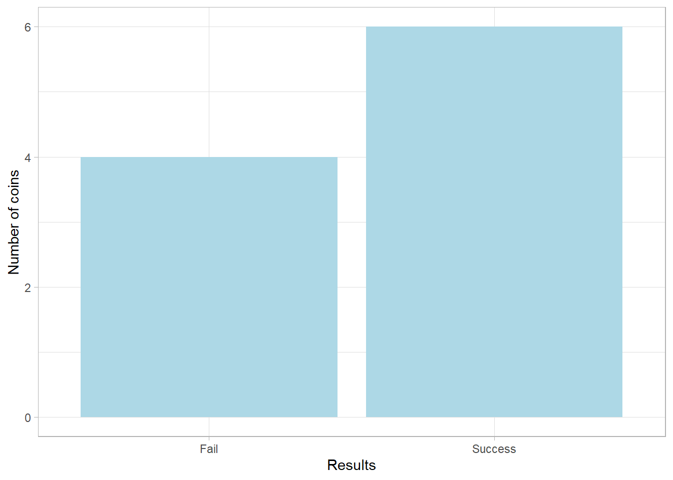
This is a Bernoulli distribution, a distribution that describes the outcome of a single trial resulting either in success (1) or failure (0). While the underlying probability of success is 50%, the bar heights in the plot might differ notably due to the small sample size. A difference of even one or two outcomes has a visible effect.
However, with a much larger sample, this variability smooths out. The Law of Large Numbers tells us that the observed proportion will converge to the true probability as the number of trials increases. Let’s simulate 10,000 coin flips to see this in action:
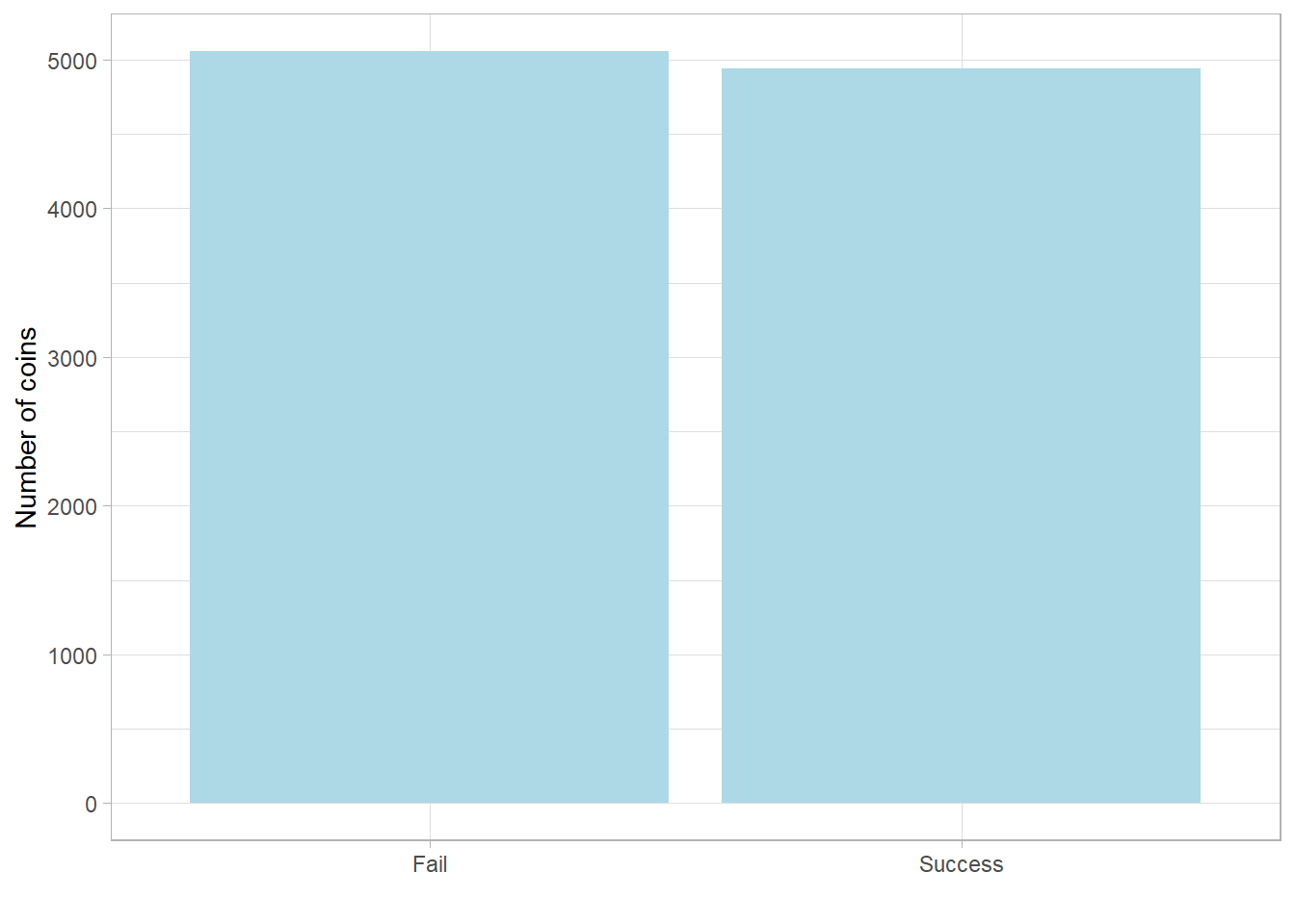
Now the two bars are nearly equal, each around 5,000, just as we would expect with a true 50% chance.
But what happens if the probability of success is not 50%? Let’s explore that by plotting Bernoulli distributions for probabilities of 20%, 50%, and 80%:
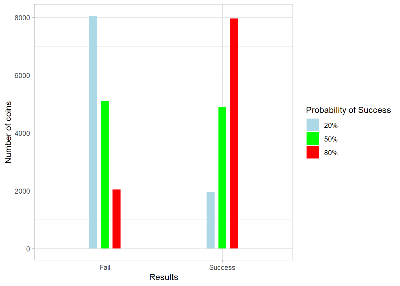
When the probability of success is 20%, around 8,000 outcomes (out of 10,000) are failures. When it is 80%, around 8,000 are successes.
12.3 What are the parameters and shape of the Bernoulli distribution?
The Bernoulli distribution is one of the simplest yet most fundamental probability distributions in statistics. It models the outcome of a single trial that results in either a success or a failure, commonly encoded as 1 and 0, respectively.
We write that a variable \(X\) follows a Bernoulli distribution using the following notation: \[ X \sim Bernoulli(p) \]Here, \(p\) is the probability of success, and it is the only parameter that defines the distribution. The probability of failure is simply \(1 - p\).
Since the Bernoulli distribution is discrete (it only takes specific values, 0 or 1), it is defined using a probability mass function (PMF), which assigns probabilities to discrete outcomes, unlike the probability density function (PDF) used for continuous distributions.
The PMF of the Bernoulli distribution is:
\[ P(X = x) = p^x (1 - p)^{1-x} \]
where \(x\) can take only the values 0 and 1 (mathematically, \(x \in \{0,1\}\)).
This compact formula handles both possible outcomes:
-
If \(x = 1\): \[ P(X = 1) = p^1 (1 - p)^{1 - 1} = p \]
-
If \(x = 0\):
\[ P(X = 0) = p^0 (1 - p)^{1 - 0} = 1 - p \]
In a Bernoulli distribution, the expected value tells us what we would get on average if we repeated the single trial many times. It is simply:
\[ E(X) = p \]
This means that if the probability of success is 0.7, the expected value is 0.7. In the long run, we expect 70% of the trials to result in success.
The variance of a Bernoulli distribution shows how much the outcomes vary around the expected value. It is calculated as:
\[ Var(X) = p(1 - p) \]
So if \(p=0.5\), then \(Var(X) = 0.5 \times 0.5 = 0.25\). This tells us that when the probability of success is balanced (like 50%), the variability is highest. If \(p\) is very close to 0 or 1, the variance is lower because the outcomes become more predictable.
Let’s relate this to our coin-flip example. If the probability of getting heads is 20%, and heads is considered a success:
-
\(P(X = 1) = p = 20\%\)
-
\(P(X = 0) = 1 - p = 1 - 20\% = 80\%\)
So, there’s a 20% chance of success and an 80% chance of failure. These values are exact probabilities, which is a key distinction of PMFs in discrete distributions. In contrast, PDFs in continuous distributions give probabilities over intervals, not exact points.
12.4 When do we encounter the Binomial distribution?
In the Bernoulli distribution, we dealt with a single trial, reviewing an example of flipping a single coin and observing whether it lands heads (success) or tails (failure). But what if we repeat this process multiple times and count the total number of successes? In this case, the resulting distribution would be a Binomial distribution.
Let’s return to our coin-flipping example. Suppose the probability of getting heads (a success) is 50%. This time, we flip 10 coins in each of 10 rounds, and in every round, we count how many heads we get.
[1] 4 6 5 7 7 2 5 7 5 5The output for each round is then shown. For example, a value of 4 means we got 4 heads out of 10 coin flips in that round. The distribution of these results can be visualized below:
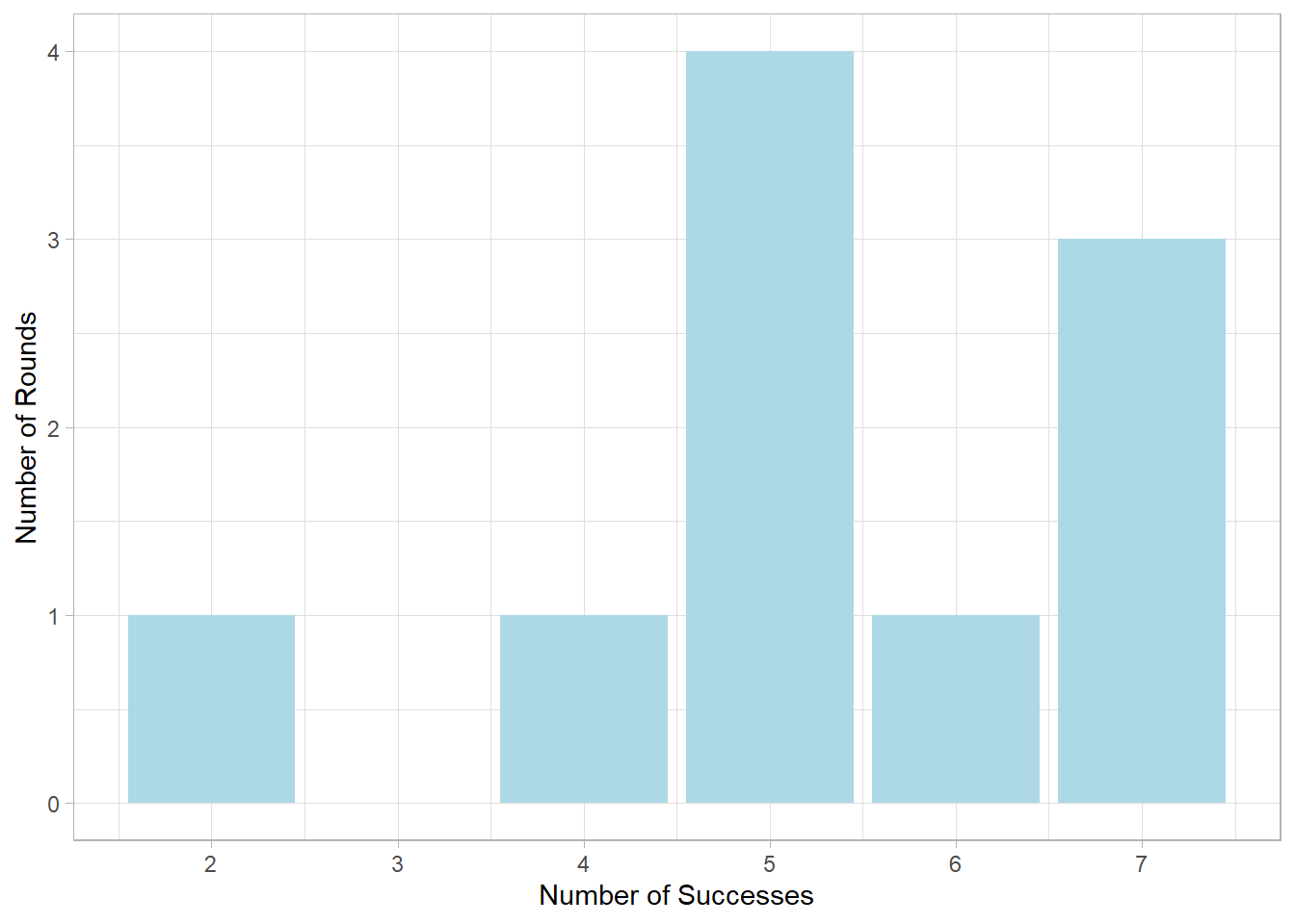
Here, the x-axis shows the number of successes (from 0 to 10), and the y-axis shows how many rounds resulted in each success count. We notice that getting 5 successes per round is quite common. That’s because the probability of success was set to 50%, so 5 out of 10 successes is the most expected outcome.
Therefore, the Binomial distribution is a distribution that counts the number of successes in a fixed number of independent Bernoulli trials.
12.5 What are the parameters and shape of the Binomial distribution?
If a random variable \(X\) follows a Binomial distribution, we write:
\[ X \sim Binomial(n, p) \]
The Binomial distribution has two parameters:
-
\(n\): the number of independent trials (e.g., number of coin flips in a round)
-
\(p\): the probability of success on a single trial (e.g., the chance of getting heads)
Because it is a discrete distribution, the Binomial distribution also uses a probability mass function (PMF) instead of a probability density function. The PMF is:
\[ P(X = x) = \binom{n}{x}p^x(1 - p)^{n - x} \]
where \(x \in \{0,1,2,...,n\}\), meaning that \(x\) can take any values from 0 up to the number of independent trials (e.g., the number of coins).
The right-hand side of the PMF is familiar from the Bernoulli distribution. It gives the probability of getting \(x\) successes and \(n-x\) failures. The added part here is the binomial coefficient, written as:
\[ \binom{n}{x} \]
This term tells us, in how many different ways we can choose \(x\) successes from \(n\) trials. In other words, it accounts for the different combinations of outcomes that lead to the same number of successes.
Factorial function
The binomial coefficient is calculated using the factorial function: \[\binom{n}{x} = \frac{n!}{x!(n - x)!}\] - \(x!\) is the number of ways to arrange the \(x\) successes. - \((n-x)!\) is the number of ways to arrange the \(n-x\) failures. This formula gives the number of unique combinations of \(x\) successes in \(n\) total trials, ignoring the order in which the successes occur. #### Example: Suppose we have 3 coins labeled A, B, and C, and we want to know how many different ways we can get heads from two out of the three coins. The valid combinations are: - A and B - A and C - B and C That’s a total of 3 combinations, and we can confirm this using the formula: \[\binom{3}{2} = \frac{3!}{2!(3-2)!}\] The value of each factorial is: - \(3! = 1 \times 2 \times 3 = 6\) - \(2! = 1 \times 2 = 2\) So: \[\binom{3}{2} = \frac{3!}{2!(3 - 2)!} = \frac{6}{2} = 3\] The factorial function helps us compute this efficiently, even when the numbers get large.
When \(n = 1\), then the Binomial distribution essentially transposes to the Bernoulli distribution. In that case, we are conducting a single trial, so the number of successes can only be 0 or 1.
Like with the Bernoulli distribution, the expected value tells us what we would get on average if we repeated the entire experiment many times. For the Binomial distribution:
\[ E(X) = np \]
This means that if you flip 10 coins with a 40% chance of heads, the expected number of heads is \(10 \times 0.4 = 4\). That doesn’t mean we will always get exactly 4 heads, it just means 4 is the long-run average number of heads over many repetitions of the experiment.
The variance of a Binomial distribution tells us how much the number of successes tends to vary around the expected value:
\[ Var(X) = np(1 - p) \]
If \(n = 10\) and \(p = 0.5\) then:
\[ Var(X) = 10 \times 0.5 \times 0.5 = 2.5 \]
This helps us understand the spread of the distribution. The further \(p\) is from 0.5, the smaller the variance becomes, as outcomes become more predictable.
To see how we can use PMF in practice, suppose we flip 10 coins (so \(n = 10\)) and the probability of getting heads is 50% (so \(p = 0.5\)), then the probability of getting exactly 6 heads is:
\[ P(X = 6) = \binom{10}{6}0.5^6(1 - 0.5)^{10-6} = 210 \times 0.5^{10} = 20.5\% \]
So, when we flip 10 coins with a probability of success of 50%, there is about a 20.5% chance of getting exactly 6 heads.
Like in the Bernoulli case, the PMF of the Binomial distribution gives us actual probabilities for each possible number of successes.
12.6 Calculating and Simulating in R
Like with Normal distribution, base R provides a family of functions to simulate and compute probabilities for the Binomial distribution. As a reminder, the key prefixes are:
-
d: for calculating the density (PMF in the case of discrete distributions). -
p: for calculating the cumulative probability (area under the curve up to a given value). -
q: for calculating the quantile (the value below which a given proportion of data falls). -
r: for random sampling (generating simulated values from the distribution).
Let’s start by simulating 10,000 independent trials of flipping 10
coins, where the probability of getting heads (success) is 30%. We
use the rbinom() function, setting
n = 10000, size = 10, and
prob = 0.3. and store the results in an object called
binomial_sim. Note that the argument n here refers to
the number of trials (how many times we repeat the 10-coin flips),
not the number of coins flipped in each trial, which is specified by
the size argument.
# Set seed
set.seed(555)

# Simulate Binomial distribution
binomial_sim <- rbinom(n = 10000, size = 10, prob = 0.3)

# View first few results
head(binomial_sim)
[1] 2 5 4 3 3 1Now, let’s visualize the distribution:
# Plot results
tibble(x = binomial_sim) %>%
  ggplot(aes(x = x)) +
  geom_bar(fill = "skyblue") +
  labs(x = "Number of Successes",
       y = "Count")
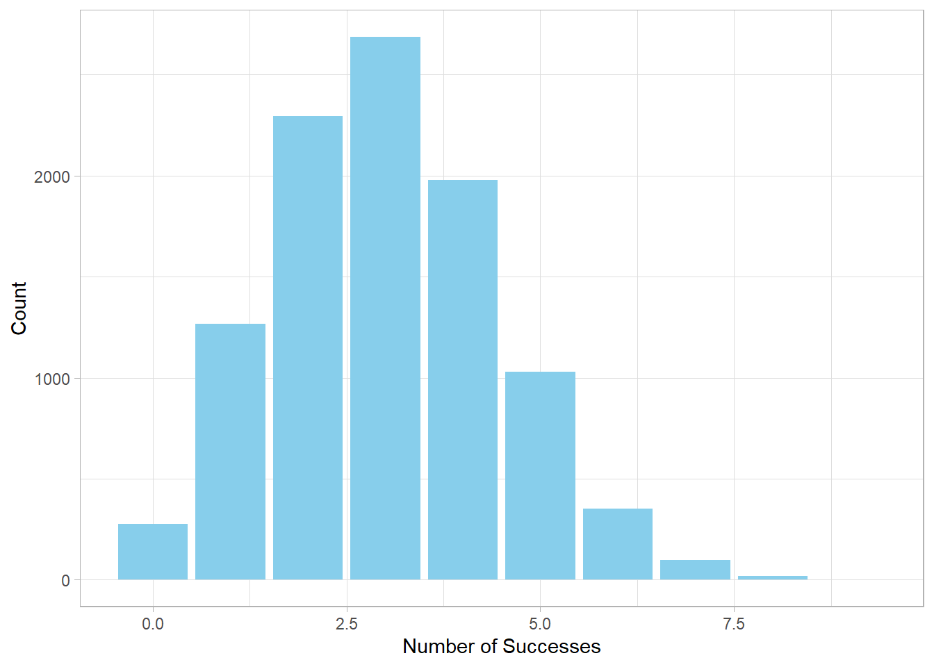
We see that the most frequent outcome is about 3 successes, which aligns with our expectation: 30% of 10 is 3.
Regarding the Bernoulli distribution, base R does not offer a
dedicated function. However, since the Bernoulli distribution is
essentially a special case of the Binomial distribution—with just a
single trial—we can use the rbinom() function with
specific argument values to simulate it.
To do this, we set the size argument to 1,
indicating that each observation consists of one trial (e.g.,
flipping one coin). The n argument, on the other hand,
specifies how many such observations we want to simulate (e.g., the
number of coins we flip).
This can feel a bit counterintuitive at first. Earlier, when working
with the Binomial distribution, size represented the
number of coins flipped in each trial, and n was the
number of repeated experiments. Now, for the Bernoulli case, we are
flipping just one coin per trial, so size = 1,
and we might want to simulate 100 such flips, which means
n = 100. In a way, we are reversing how we think about
these two arguments.
By setting size = 1 and n = 100, we’re
effectively simulating 100 independent Bernoulli trials, each with
one coin flip:
# Set seed
set.seed(555)
# Simulate Bernoulli distribution
bernoulli_sim <- rbinom(n = 100, size = 1, prob = 0.3)
# View first few results
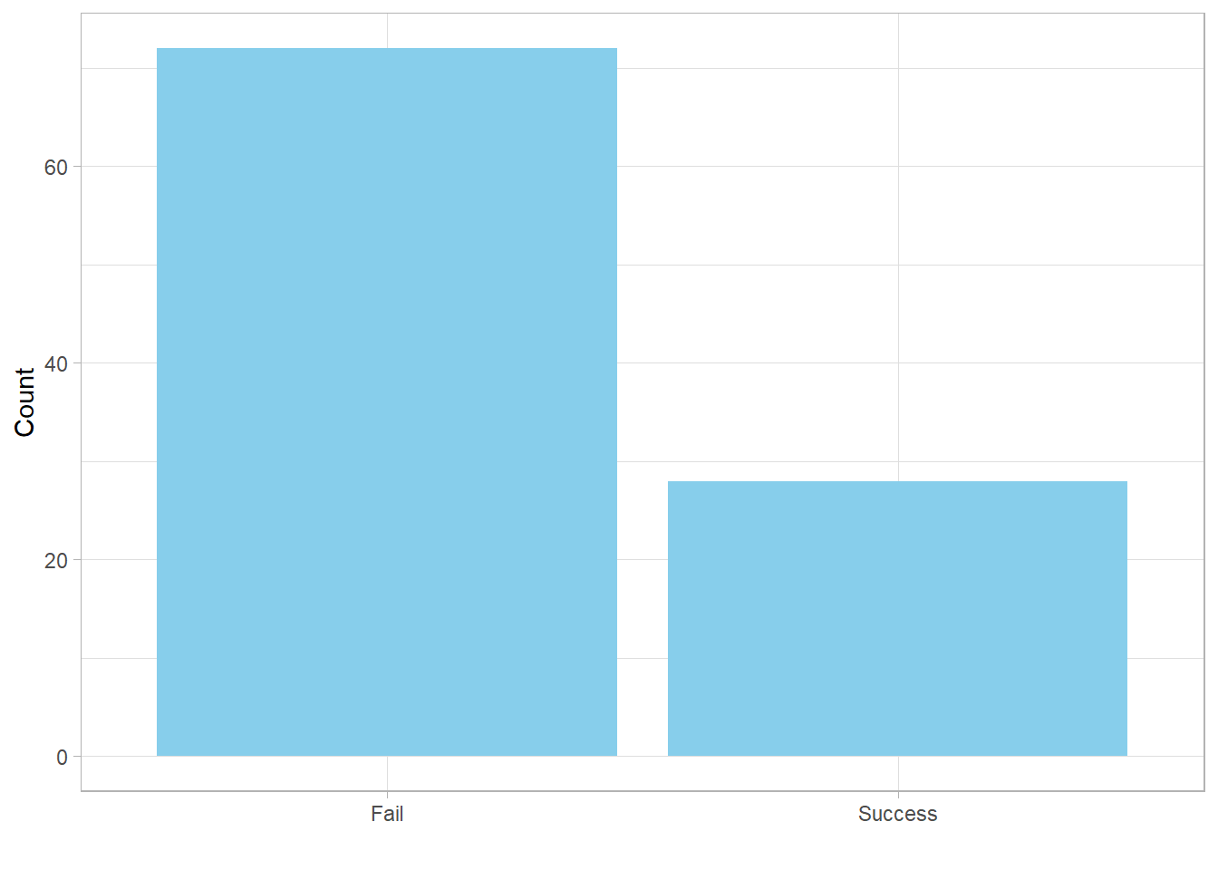
head(bernoulli_sim)[1] 0 1 0 0 0 0We can also visualize the result:
# Plot results
tibble(x = bernoulli_sim) %>%
  mutate(Label = if_else(x == 1, "Success", "Fail")) %>%
  ggplot(aes(x = Label)) +
  geom_bar(fill = "skyblue") +
  labs(x = "", y = "Count")
As discussed earlier, the probability mass function (PMF) allows us to directly calculate the probability of observing a specific number of successes, given a certain number of trials and a fixed probability of success for each trial.
For example, suppose we want to find the probability of getting
exactly 3 successes in 10 coin tosses, where the probability of
success on each toss is 30%. We can use the
dbinom() function in R for this purpose, setting
size = 10 and prob = 0.3:
# Calculate probability of getting 3 successes using PMF
dbinom(x = 3, size = 10, prob = 0.3)
[1] 0.2668279The result tells us that the probability of getting exactly 3 successes is approximately 26.69%. This aligns with the theoretical PMF formula:
\[ P(X = 3) = \binom{10}{3}0.3^3(1 - 0.3)^{10-3} = \binom{10}{3} 0.3^3 0.7^7 \approx 26.6\% \]
PMF vs Expected Value
It’s important not to confuse the PMF with the expected value. The PMF gives the probability of a specific outcome, such as getting exactly 3 successes in 10 trials. In our case, that’s about 26.69%. The expected value, on the other hand, is the long-run average number of successes. It’s calculated as: \[ E(X) = n \times p = 10 \times 0.3 = 3 \]
This means that, if we repeat the experiment many times, the average number of successes will be around 3.
Since we’ve already simulated this scenario using
binomial_sim, and our data is discrete, we can estimate
this same probability empirically. To do that, we count how many of
the 10,000 simulations resulted in exactly 3 successes and divide by
the total number of trials:
# Calculate probability of getting 3 successes using binomial_sim
sum(binomial_sim == 3) / length(binomial_sim)
[1] 0.2686This empirical result should be close to the theoretical probability of 26.69%.
Next, the pbinom() function allows us to compute
cumulative probabilities, meaning the probability of getting
up to and including a certain number of successes. The only
difference from dbinom() is that the argument is called
q instead of x. For example, to calculate
the probability of getting 3 or fewer successes:
# Calculate cumulative probability of getting at most 3 successes
pbinom(q = 3, size = 10, prob = 0.3)
[1] 0.6496107
To verify this with our simulation, we calculate the proportion of
trials in binomial_sim where the number of successes is
less than or equal to 3:
# Estimate cumulative probability from simulation
sum(binomial_sim <= 3) / length(binomial_sim)
[1] 0.6524Again, the simulation should closely match the theoretical result.
Finally, the qbinom() function allows us to work in the
reverse direction: it finds the
smallest number of successes such that the cumulative
probability is at least a given value. For instance, if we want to
determine the minimum number of successes needed to cover at least
60% of the distribution:
# Find the quantile that corresponds to the 60th percentile
qbinom(p = 0.6, size = 10, prob = 0.3)
[1] 3This result makes intuitive sense: earlier, we saw that up to 3 successes captured approximately 65% of the distribution, while up to 2 successes only captured about 38%. Thus, 3 is the smallest number of successes where the cumulative probability exceeds 60%.
12.7 From Binomial to Normal
In our earlier example, we used a 30% chance of success, which resulted in a right-skewed distribution. If we had used 70% instead, the distribution would be left-skewed. However, in many real-world scenarios—like tossing a fair coin—the probability of success is 50%.
Let’s revisit the simulation, this time using a larger number of trials (100 coins) and setting the probability of success to 0.5:
# Set seed
set.seed(555)

# Simulate Binomial distribution
binomial_sim <- rbinom(n = 10000, size = 100, prob = 0.5)

# Plot results
tibble(x = binomial_sim) %>%
  ggplot(aes(x = x)) +
  geom_bar(fill = "skyblue") +
  labs(x = "Number of Successes",
       y = "Count")
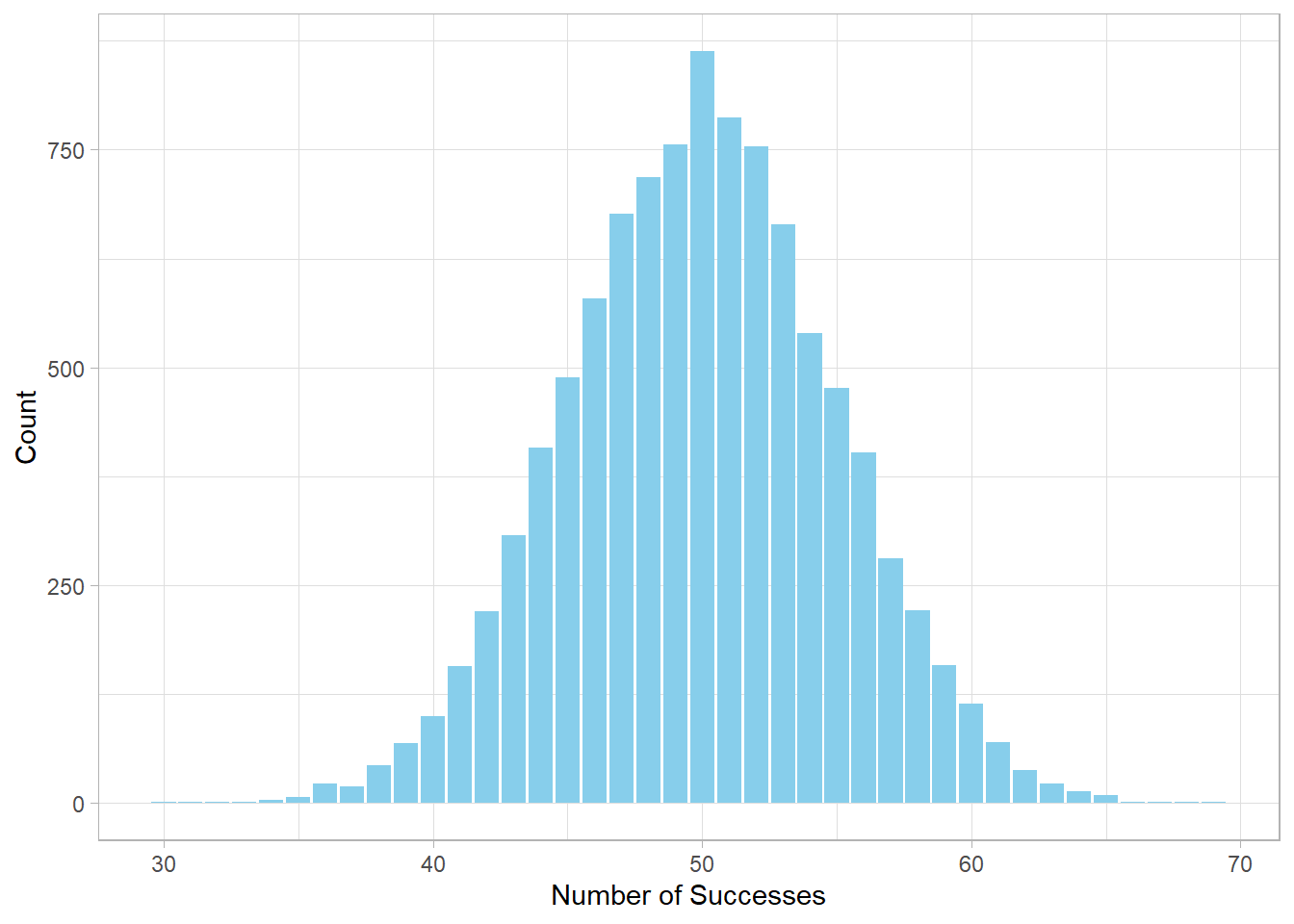
The resulting distribution is symmetric and bell-shaped, closely resembling the Normal distribution. This is not a coincidence. According to the Central Limit Theorem, when the number of trials is large and the probability of success is not too close to 0 or 1, the Binomial distribution tends to resemble a Normal distribution.
To illustrate this, let’s compute the probability of getting 40, 50, and 55 successes using the Binomial PMF:
# Calculate the exact binomial probability of getting 40 successes
dbinom(40, size = 100, prob = 0.5)
[1] 0.01084387# Calculate the exact binomial probability of getting 50 successes
dbinom(50, size = 100, prob = 0.5)[1] 0.07958924# Calculate the exact binomial probability of getting 55 successes
dbinom(55, size = 100, prob = 0.5)[1] 0.0484743Despite 50 being the most likely outcome, the probability is only around 8%. With so many possible combinations, individual probabilities become quite small, even for central values.
Earlier, we discussed the formulas for the expected value and variance of a Binomial distribution. Let’s now compute them:
# Expected value: n*p
expected_value <- 100 * 0.5

# Expected value
expected_value
[1] 50# Variance: n*p*(1-p)
variance <- 100 * 0.5 * (1 - 0.5)
# Print variance
variance[1] 25Using these values, we can now estimate the likelihood of 40, 50, and 55 successes using the Normal distribution:
# Calculate the normal approximation of getting 40 successes
dnorm(40, mean = expected_value, sd = sqrt(variance))
[1] 0.01079819# Calculate the normal approximation of getting 50 successes
dnorm(50, mean = expected_value, sd = sqrt(variance))[1] 0.07978846# Calculate the normal approximation of getting 55 successes
dnorm(55, mean = expected_value, sd = sqrt(variance))[1] 0.04839414
Comparing these values with the results from
dbinom() confirms our point: when the number of trials
is large and the probability of success is moderate, the Binomial
distribution closely resembles the Normal
distribution.
12.8 Recap
The Bernoulli distribution is a fundamental building block in probability and statistics. It models situations with only two possible outcomes, such as success or failure, yes or no, true or false. Understanding the Bernoulli distribution helps us grasp more complex concepts such as the Binomial distribution, which extends the idea to multiple repeated trials.
When the number of trials in a Binomial distribution becomes large, the Binomial can be closely approximated by the Normal distribution. This approximation is useful because the Normal distribution is mathematically easier to work with and appears frequently in real-world data. This connection shows how the simple Bernoulli process links to broader, more complex statistical models.