log(16, base = 2)[1] 4Suppose you are a forest ranger tasked with monitoring the growth of trees in a forest reserve. When you begin, the forest contains 100 trees. Over the next four years, you observe that the number of trees doubles each year:
Although the percentage change remains constant - each year the number of trees increases by 100% - the actual number of new trees grows exponentially: 100 new trees in the first year, 200 in the second, 400 in the third, and so on.
Of course this is a hypothetical example. In practice, forests don’t grow precisely like that.
This type of growth can be expressed using an exponential function, as follows:
\[N = 100 \times 2^t\]
where \(N\) is the number of trees and \(t\) is the number of years.
This formula makes it easy to predict the number of trees at any future time point. For example, after two years, the expected number of trees will be: \[N = 100 \times 2^2 = 100 * 4 = 400\]
However, suppose we reverse the question: In how many years will there be 6.400 trees? We must solve for \(t\) in the equation: \[6.400 = 100 \times 2^{t}\]
To isolate \(t\), we use logarithms. Taking base-2 logarithms of both sides: \[log_26400 = log_2(100 * 2^t)\] \[log_26400 = log_2(100) + log_2(2^t)\] \[log_26400 = log_2(100) + t\]
Solving for \(t\), we have: \[t = log_26400 - log_2100\] \[t = log_2(\frac{6400}{100})\] \[t = log_2(64)\] \[t = 6\]
Thus, the forest reaches 6.400 trees after six years. In this example, the logarithm allows us to solve an equation in which the unknown appears in the exponent.
This illustrates one of the most important uses of logarithms: solving equations involving exponential growth. Logarithms have broad applications in Data Science, Finance, Biology, Medicine, and many other fields. Yet, while many people know that \(log_22 = 1\), they may not fully understand the utility of logarithms. This chapter introduces the intuition and mathematical properties of logarithms and demonstrates their practical value, within the Data Science context.
Logarithms were developed by John Napier and Henry Briggs to… simplify calculations. By converting multiplication into addition and division into subtraction, logarithms offered a powerful computational shortcut in the pre-digital era. For instance, instead of multiplying 32 by 16 directly, we express both as powers of 2:
Then: \[32 \times 16 = 2^{5} \times 2^{4} = 2^{9}\]
Before we discuss the mathematical properties of logarithms, it is important to understand the terminology. Suppose we have the following mathematical equation: \[2^{4} = 16\]In this equation, number 4 is called power, exponent or index, and number 2 is the base. If we have \(3^{4} = 81\), then we say that number 3 is the base and number 4 is the power(or exponent or index).
Suppose we have the following equation: \[16 = 2^{4}\]
This equation is equivalent to: \[log_216 = 4\]
We describe this equation as ‘log to base 2 of 16 equals 4’. We can confirm this result in R by using the following code:
log(16, base = 2)[1] 4The subscript of a log shows the base (“2”) and the result (“4”) is the power of that base that leads to the number (“16”) of the log. This is what we used in the introduction example, in which we asked in which year we will have \(N\) number of trees. In other words, to which power do we need to raise the base 2 in order to have a result of 16? The answer is 4. More generally, we have the following mathematical equation:
\[x = a^{n} \Leftrightarrow log_ax = n\]
A special case of this property is \(a = a^{1}\). We know that this equation holds and, as a result, we can conclude that: \[log_aa = 1\] We can see that this is the case when using R to do the calculation:
# a = 10
log(10, base = 10)
[1] 1# a = 2
log(2, base = 2)[1] 1Therefore, when we use logs, we essentially “pivot” on the base of a number; that number was the value of 2 in our tree example.
We saw that: \[x = a^{n} \Leftrightarrow log_ax = n\]
Assume that instead of \(x = a^{n}\), we had: \[x^{z} = (a^{n})^{z} \Leftrightarrow x^{z} = a^{n + z}\]
By taking the log of that equation, we have: \[log_ax^{m} = log_aa^{nm} = nm\]We know that \(log_aa^{nm} = nm\) because if we raise the base \(a\) to the power of \(nm\), the result would be \(a\) to the power of \(nm\).
Since we saw earlier that \(log_ax = n\), we can conclude that the following property holds: \[log_ax^{m} = m \times log_ax\]
Suppose we have the following two equations:
Did you notice that the base on the right hand side is the same number? If we want to multiply numbers x and y, then we have: \[xy = a^{n} \times a^z = a^{(n + z)}\]
From the property of logarithms we previously explained, we have the following:
\[xy = a^{(n + z)} \Leftrightarrow log_axy = n + z\]
At the same time, if we apply the previous property in each of the two equations separately, we get:
\[x = a^{n} \Leftrightarrow log_ax = n\] and \[y = a^{z} \Leftrightarrow log_ay = z\]
Therefore, we can conclude that the following property holds:
\[log_axy = n + z \Leftrightarrow log_axy = log_ax + log_ay\]
Similarly, suppose we have (again) the following two equations:
This time, we want to divide \(x\) by \(y\). We have: \[\frac{x}{y} = \frac{a^{n}}{a^{z}} = a^{n - z}\] Respectively, from the first property of logarithms we discussed, we have the following: \[\frac{x}{y} = a^{n - z} \Leftrightarrow log_a\frac{x}{y} = log_a{a}^{n - z} \Leftrightarrow log_a\frac{x}{y} = n - z \] As we did previously, we can apply logs to each of the initial equations separately:
\[x = a^{n} \Leftrightarrow log_ax = n\] and \[y = a^{z} \Leftrightarrow log_ay = z\]
Therefore, we can conclude that the following property holds:
\[log_a\frac{x}{y} = n - z \Leftrightarrow log_a\frac{x}{y} = log_ax - log_ay\]
Suppose we have the following two logarithms:
For the first, we understand that we need to raise the base 9 to the power of 1/2 (which is equivalent to the square root) in order to get 3. For the second, we see that we need to raise the base 3 to the power of 2 in order to get 9.
More broadly, it becomes evident that we can substitute the denominator of the right hand side of the first equation with the left hand side of the second equation. We therefore have: \[log_93 = \frac{1}{log_39}\]
Trying this with different numbers, the conclusion will always be the same. Thus, the following mathematical equation: \[log_ab = \frac{1}{log_ba}\]
The two most common bases are 10 and e. A log without a specific base implies that its base is 10. However, in R, the function log has e as its base. Since we know that \(log_{10}10 = 1\), let us confirm this by using the following code.
# Specify the base
log(10, base = 10)
[1] 1# Not specify the base
log(10)[1] 2.302585The exponential constant e is a special number—about 2.71828—that naturally appears when things grow continuously, such as populations, interest, or radioactive decay. It is the base of natural growth processes and is very important in applications across physics, biology, and other fields. Logarithms with base e are usually written as ln and are called natural logarithms.
From our high school years, we may remember that any number \(a\) that is raised to the power of 0 is 1. So, \(a^{0} = 1\). The logarithm in this cases is: \[log_{a}1 = 0\]
In those cases, the base of a logarithm does not matter; any number that is raised to the power of 0 is 1.
One question that may arise is “What about 0 or negative numbers?”. Indeed, we cannot take the logarithm of a non-positive number, including 0, using the standard logarithmic functions such as the natural logarithm (\(ln\)) or the common logarithm (log with base 10). This is because the logarithm function grows infinitely negative as its input approaches 0 from the positive side. Let us confirm this in R by using the following code:
log(0)[1] -InfThus far we learned (or reviewed) the basic mathematical properties and intuition behind logarithms. However, we still have not discussed how and why we would use logarithms in practice. In other words, why are logarithms (logs) useful in fields such as Data Science? Although the trick that we replace multiplication with addition seems smart, nowadays we have computers and calculators that can solve much more complicated formulas. Indeed, we can use logarithms for many different purposes, but let us explain below two of their most prominent and important applications. ### Relative difference
Suppose that we have a variable describing yearly salary. The distribution of that variable can be seen in the plot below:
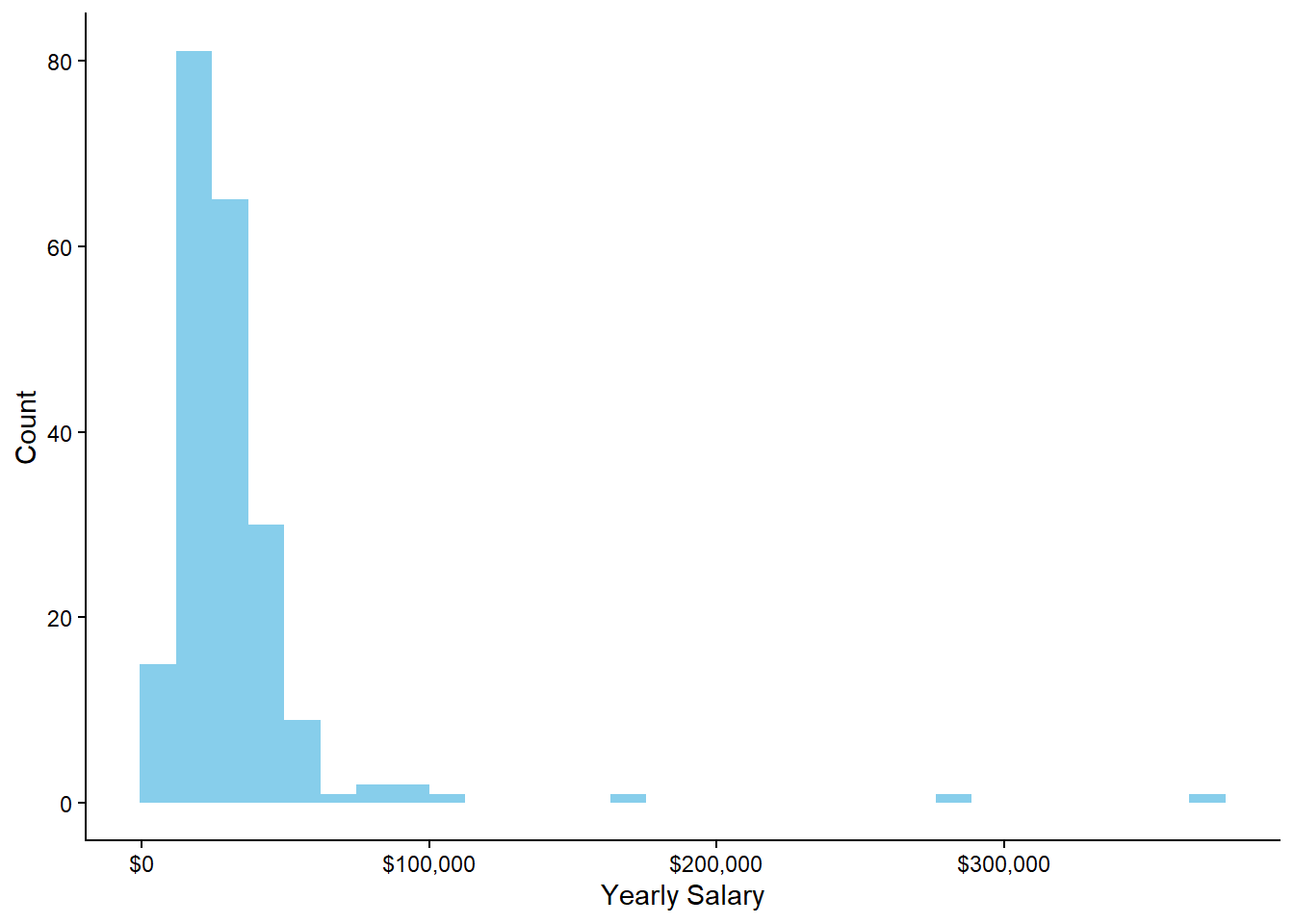
This distribution is slightly positively skewed, meaning that there are some extreme values on the positive side of the x-axis that “pull” the center of the distribution (remember, the mean is affected by outliers).
However, we know that if we had a Normal Distribution and Central Limit Theorem, things would be much easier for us, as using it makes our work much easier and more intuitive.
By using log transformation, the values of variable \(x\) change, meaning that the shape of the distribution now is different:
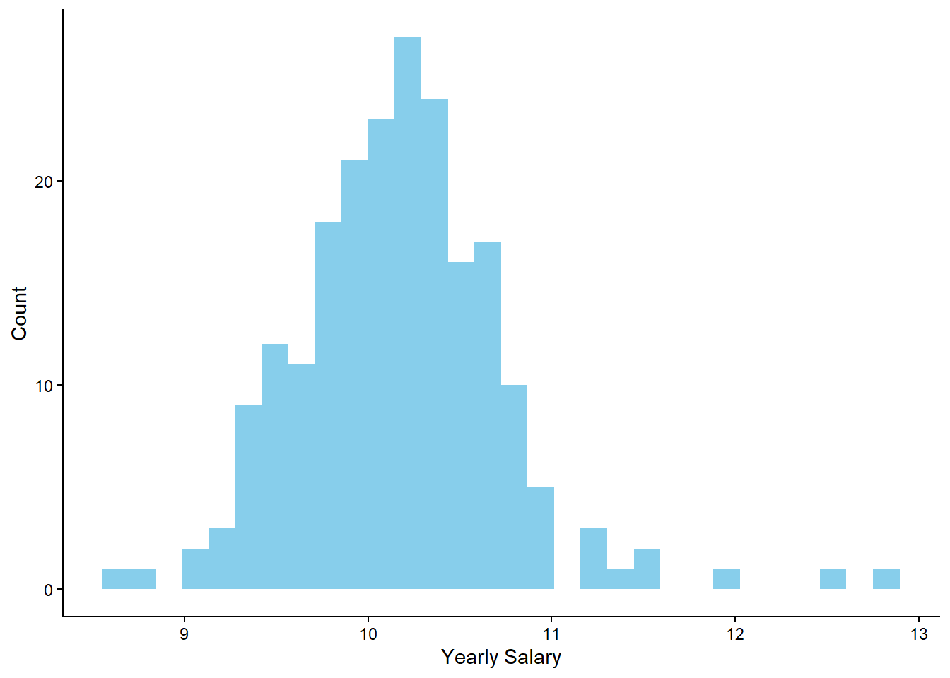
The distribution looks slightly more normal (the extreme values are closer to the center of the distribution) and, as a result, we could use this new distribution to perform our statistical analysis. We also see that the values on the x-axis are different, since we use logs and not the raw values.
The reason of such transformation is that we are interested in the relative difference among the values. For example, the difference between $80,000 and $100,000 is the same as the difference between $100,000 and $120,000. However, the relative difference is different: going from 80,000 to 100,000 is a 25% change while from 100,000 to 120,000 is a 20% change.
Variables such as salaries almost always demonstrate positively skewed distributions. In these cases, it is highly recommended to use the log of these variables when we analyze a data set. This type of distributions is called log-normal, because their shape changes to that of normal when we apply log transformation.
Another useful property is the one that we discussed in the introduction example with the growth of the number of trees in the forest. In that example, we mentioned that the percentage change is constant and that the number of trees grows exponentially. For simplicity, we create the following data frame:
# Data frame
data <- data.frame(Year = 0:10,
                   Number_of_Trees = 50 * cumprod(rep(2, 11)))

# Print the data frame
data
Year Number_of_Trees
1 0 100
2 1 200
3 2 400
4 3 800
5 4 1600
6 5 3200
7 6 6400
8 7 12800
9 8 25600
10 9 51200
11 10 102400
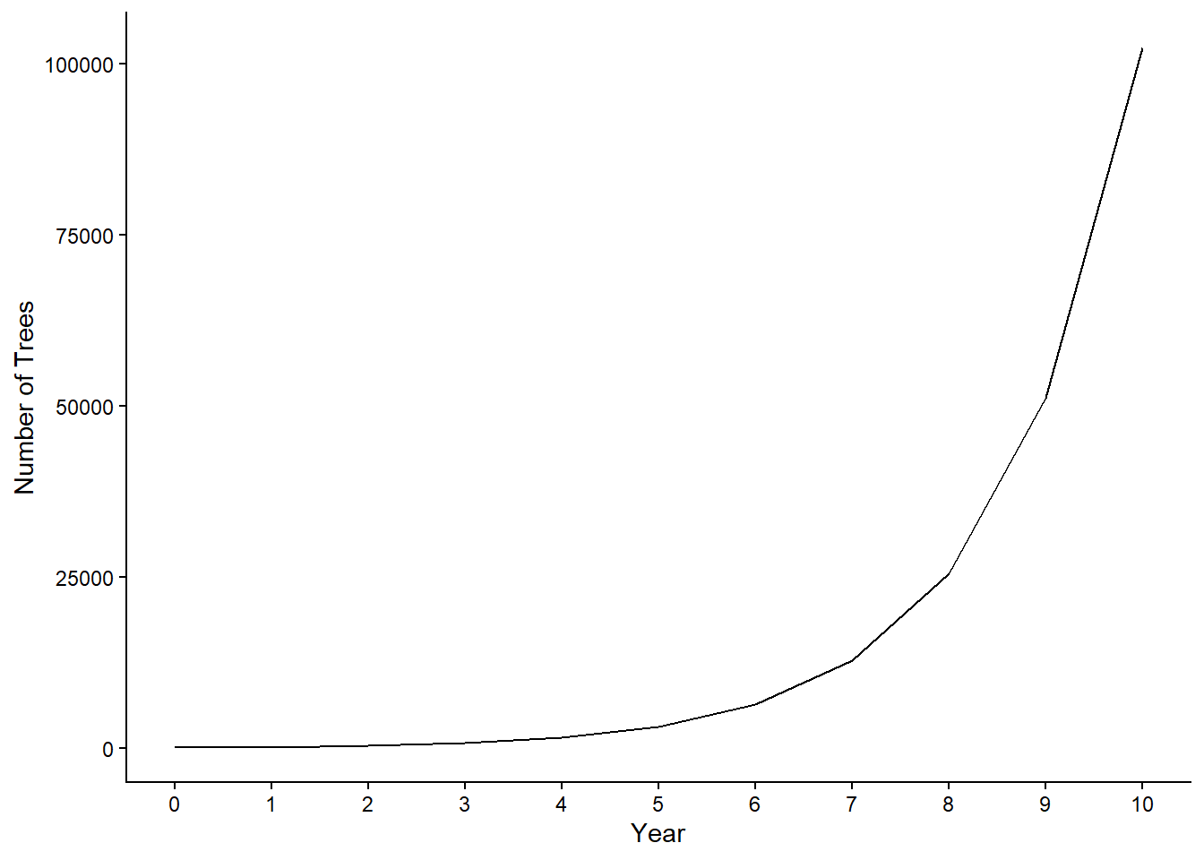
The number of trees grows exponentially across the years, meaning that, as time passes, more and more trees grow. However, the growth rate remains steady. Remember, the number of trees always doubles (100% increase from one year to the other). If we take the log of the number of trees, the plot looks different:
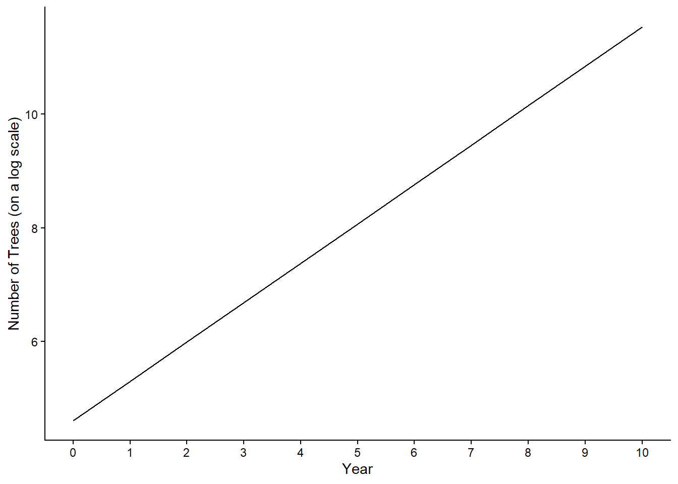
With logs, we transform (or, in a sense, simplify) exponential growth into a linear relationship, making it easier to analyze and understand the progression of the population (trees). For instance:
Year 1: 200 trees \(log_2200 \approx 7.643\)
Year 2: 400 trees \(log_2400 \approx 8.644\)
Year 3: 800 trees \(log_2800 \approx 9.643\)
We therefore have a constant increase by 1 unit on the logarithm scale. This is intuitive, because we just multiply the number of trees of the previous year by 2 and remember that the result of a log is the power of a base.