9  Scaling

9.1 Introduction

In this chapter we discuss the concept of scaling. In most cases, the purpose of scaling a variable is twofold: first, we can easily check by how much an individual value differs from the center of its distribution as compared to its other values, especially when the unit of measurement is not intuitive. An example to consider would be in the pharma industry, where a drug is measured in micrograms or nanograms, making raw numeric differences hard to interpret without some form of transformation. Second and, more importantly, scaling makes different variables or groups directly comparable, especially when they have different units, ranges, or variances. Scaling helps us interpret values relative to their own distribution and compare them on a consistent basis.

To understand why this is an important concept, let’s consider a simple example. Suppose we take two university courses, A and B, and our final grades are 8.5 out of 10 and 18 out of 20, respectively. At first glance, we might argue that we performed better in course B—after all, 18 out of 20 is equivalent to 9 out of 10, which is slightly higher than our grade in course A. However, this comparison overlooks a crucial detail: the behavior of other students in each course. What if most students in course B scored 19 or 20, while students in course A generally scored around 6.5 or 7? In that case, our 8.5 in course A would be well above average, while our 18 in course B would actually be below average.

This is where scaling becomes useful. Instead of comparing raw grades, we could scale each one relative to its own distribution, meaning we take into account the mean and variability of grades in each course. This way, we’re not comparing the courses directly, but comparing how well we performed within each course. In essence, scaling transforms a variable so that values reflect their position within a distribution, rather than their absolute magnitude. Nonetheless, scaling does not change the shape of the distribution of the variable; it only removes the units of measurement.

Even though there are different scaling methods, we will focus on the following three in this chapter:

• Centering

• Min-Max scaling (Normalization)

• Standardization

Each of these methods transforms the variable in a different way, and is most plausibly applicable depending on our goal at hand. Such a goal can be to remove the average (centering), constrain values to a specific range (min-max scaling), or to standardize differences based on variation (standardization).

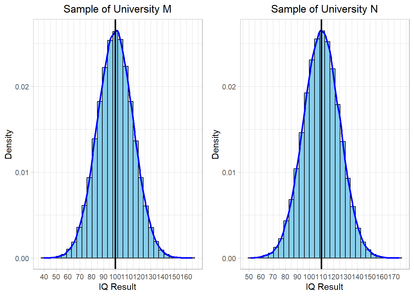
To see how each method works in practice, let’s assume we have collected two samples from two universities: University M and University N. These samples reflect IQ test results of students and both follow a normal distribution. The average IQ in the first sample (University M) is 100, while the average in the second sample (University N) is 110. In both cases, the standard deviation is 15. The distributions of these two samples are visualized below:

These two samples have the same bell-curved shape and variability (standard deviation), but they differ in their center values, as shown by the vertical black lines. University M has an average IQ of 100, and University N has an average IQ of 110.

We will now apply each scaling method to these distributions to see what changes, what remains the same, and how scaling helps us make meaningful comparisons across samples.

9.2 Scaling Methods

9.2.1 Centering

The first scaling method we will look at is centering. This is one of the simplest methods: we subtract the average value (the mean) of the variable from each individual value. The result tells us how far each observation is from the mean of its distribution.

Mathematically, this transformation is expressed as:

\[ x_{centered} = x - \bar{x} \]

where \(x\) is an individual value, \(\bar{x}\) is the mean of the variable, and \(x_{centered}\)​ is the new, centered value.

Centering is useful when we are interested in how values deviate from the average, especially when comparing two distributions that have similar shapes but different centers. It allows us to remove the influence of the mean and focus on the relative differences within each group.

To see how centering affects our earlier IQ data, we apply this method to the two university samples and visualize the results:

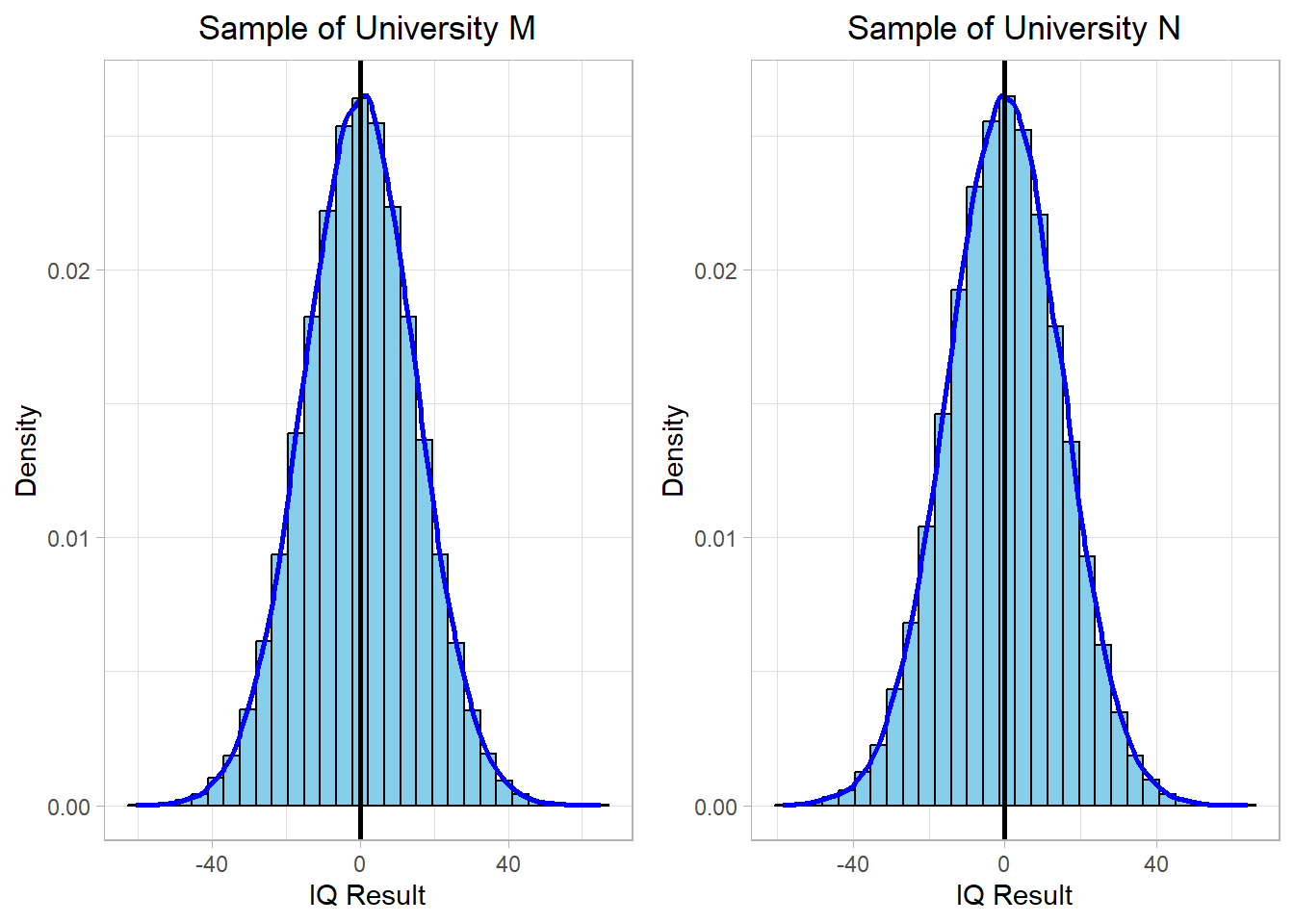
After centering, both distributions are now aligned so that their means are at zero. A student from University M who scored 100, which is exactly the mean of his or her group, now has a centered value of 0. The same goes for a student from University N who scored 110.

If we had only looked at the raw IQ scores, we might have concluded that the University M student performed worse (comparing to their peers). But after centering, we see that both students performed exactly at the average level within their respective groups. Centering removes the influence of differing means and allows for fairer within-group comparisons.

9.2.2 Min-Max Scaling

Another common scaling technique is min-max scaling, also known as normalization. This method transforms all values in a variable so that they lie within a specific range, typically between 0 and 1. It is particularly useful when we want to ensure that all variables contribute equally to the analysis, regardless of their original scales.

Definition

The term normalization is sometimes used in two ways. In many practical settings, it refers specifically to min-max scaling, but in other cases, it’s used more broadly to mean any kind of scaling or rescaling that helps make data comparable.

The formula for min-max scaling is:

\[ x_{scaled} = \frac{x - x_{min}}{x_{max} - x_{min}} \]

where:

• \(x\) is an individual value,

• \(x_{min}\)​ is the minimum value in the variable,

• \(x_{max}\) is the maximum value, and

• \(x_{scaled}\) is the scaled (new) value.

This transformation resizes the entire distribution so that the smallest value becomes 0 and the largest becomes 1. Values in-between are rescaled proportionally.

We now apply min-max scaling to the IQ samples from both universities and visualize the result:

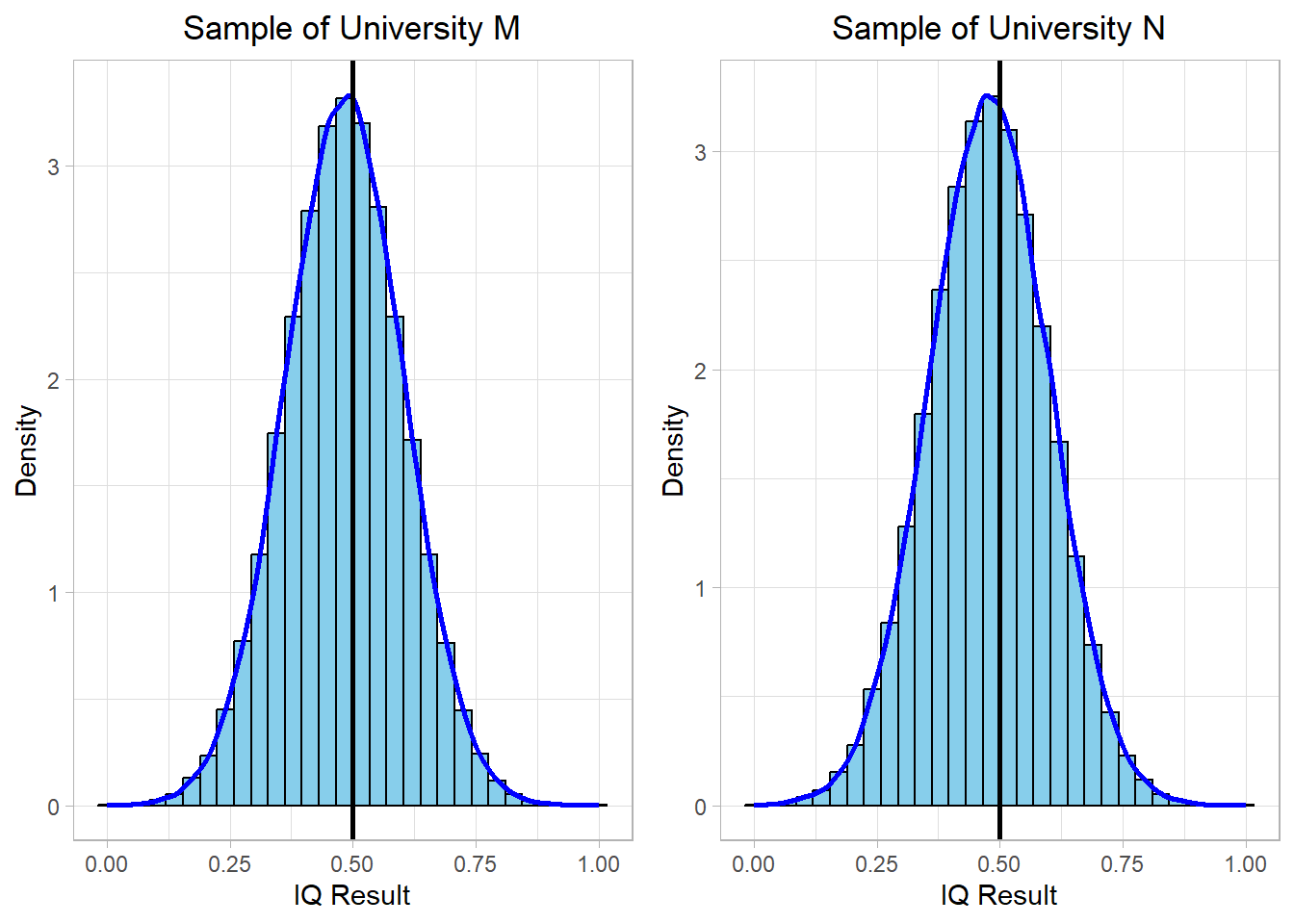
After applying min-max scaling, both distributions are rescaled to fit within the [0, 1] range. The vertical (black) line at 0.5 represents the midpoint of this new scale. While the shape of each distribution remains unchanged, their raw units are removed, and the values are now expressed relative to the minimum and maximum in each sample.

This technique is especially helpful when comparing variables that originally had very different ranges. However, one limitation of min-max scaling is that it is sensitive to outliers, meaning extreme values can stretch the range and compress the majority of the data into a narrow interval.

In our case, both university IQ samples had similar shapes and ranges, so the distributions after min-max scaling remain comparable. Yet, it’s important to keep in mind that this method focuses on range-based comparison rather than distance from the mean, in contrast to centering.

9.2.3 Standardization

Standardization, also known as z-score scaling, is another widely used method for transforming a variable. Unlike min-max scaling, which rescales the data to a specific range, standardization rescales data based on the mean and standard deviation of the variable. This transformation expresses each value in terms of how many standard deviations it is away from the mean.

The formula is:

\[ x_{standardized} = \frac{x - \bar{x}}{s} \]

where:

• \(x\) is an individual value,

• \(\bar{x}\) is the mean of the variable,

• \(s\) is the sample standard deviation and

• \(x_{standardized}\) is the standardized value (or z-score).

After standardization, the transformed variable has a mean of 0 and a standard deviation of 1. This makes it easier to compare variables with different units or distributions, and to identify extreme values (outliers).

Let’s now apply standardization to the IQ samples from both universities and visualize the result:

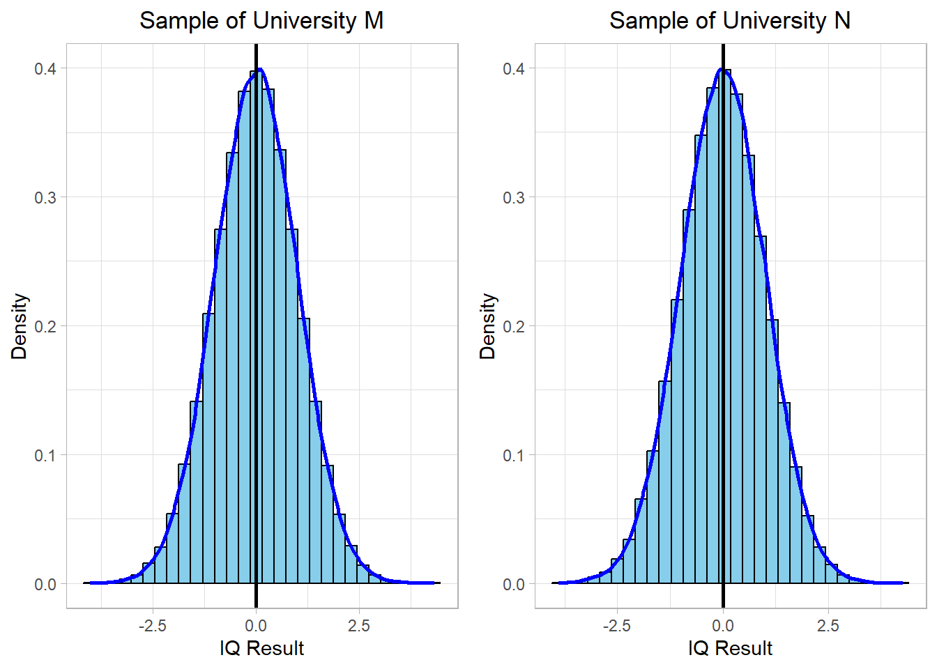
After applying standardization, both distributions are now centered around 0, and the units have been converted to standard deviations. A z-score of 0 means that the value is exactly at the mean, while a z-score of +1 or −1 indicates that the value is one standard deviation above or below the mean, respectively.

This is particularly useful when comparing values across different distributions. For example, a University M student with an IQ of 115 and a University N student with an IQ of 125 may appear different in raw scores, but if both correspond to a z-score of +1, we know they are similarly above average within their own institutions.

Standardization is a robust method, especially in statistical models and machine learning algorithms that assume variables are on the same scale. It maintains the shape of the distribution and highlights relative standing rather than absolute values.

9.3 Comparison of Scaling Methods

Now that we have explored centering, min-max scaling, and standardization, let’s compare them side by side to understand when to use each and what effect they have on the data.

All three methods transform the data without changing its overall shape. That means the distribution of the values remains the same. What changes is the position of the data (in terms of center and range) and, in some cases, its interpretability or suitability for different analyses.

The following table summarizes the key differences:

Method	Mean After Scaling	Range After Scaling	Affected by Outliers?	Keeps Distribution Shape
Centering	0	Same as original	No	Yes
Min-Max Scaling	Between 0 and 1	0,1	Yes	Yes
Standardization	0	Based on SD (~ -3 to +3)	Can be affected	Yes

9.4 Final thoughts

Scaling might seem like a minor technical detail, but it plays a significant role in how we understand and compare data. It doesn’t change the shape of the distribution or the story behind the numbers, but it makes that story easier to read and - sometimes - articulate.

Each method we’ve discussed has its own purpose. Centering shows how far values are from the average. Min-max scaling brings everything into the same range so we can compare values directly. Standardization helps us understand how unusual or typical a value is within its own group.

Choosing the right method depends on what we’re trying to accomplish. Sometimes we want to focus on how far some observation is from the average. Other times we want to put all observations on the same scale to make comparisons fair. And in many cases, we just want to prepare our data for analysis in a way that avoids measurement bias.

In the end, scaling helps us work with data more clearly and fairly. It’s a simple tool, but one that can make a real difference in how we draw conclusions and make decisions.