15 Gamma and Exponential Distributions
15.1 Introduction
In the previous chapter, we explored two discrete distributions: the Poisson and the Geometric. These distributions help us understand the behavior of rare events, such as how many times something happens in a given interval (Poisson) or how long we have to wait until the first success (Geometric).
In this chapter, we move from the world of discrete outcomes to the world of continuous time. More specifically, we focus on the Gamma distribution and the Exponential distribution. Both distributions are used in situations where events happen randomly but consistently over time, such as the time between customer arrivals at a service desk, the time between failures of machines, or the lifespan of electronic components.
If we think of the Geometric distribution as the number of failures before the first success, the Exponential distribution is its continuous-time analogue: it tells us how long we wait before the first event occurs. Similarly, the Gamma distribution generalizes the Exponential distribution by modeling the time until a number of events happen.
Throughout this chapter, we’ll explore when and why to use these distributions, how to understand their parameters, and how to simulate and visualize them in R. Whether we model service times, failure times, or inter-arrival durations, these tools give us a flexible way to handle randomness in continuous time.
15.2 When do we encounter the Gamma distribution?
Suppose we have already observed 2 customers arriving at a store, and now we want to know how long we can expect to wait until the third customer arrives. This kind of problem is where the Gamma distribution becomes very useful. The Gamma distribution models the total waiting time until the \(k^{th}\) event in a process where events happen at a steady average rate and independently of each other. Since time is continuous and positive, the Gamma distribution is well suited for modeling waiting times, lifetimes of devices, or service durations.
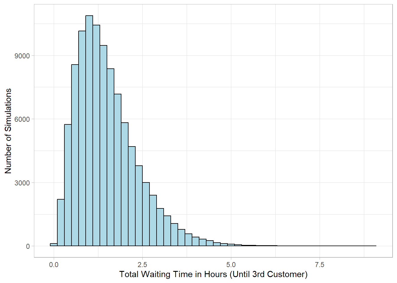
In our example, if on average 2 customers arrive at the store per hour and we have already observed that 2 customers have already visited the store, the probability distribution below shows the total waiting time it takes for the third customer to arrive, assuming customer arrival times are independent and follow the same average rate.
Note that the values on the x-axis represent the total waiting time from the beginning of the observation period until the third customer arrives. So, for example, a value of 0.5 means that all three first customers arrived within the first 30 minutes. A value of 2 means the third customer arrived after two full hours (again from the beginning of the observation period). The Gamma distribution captures the randomness of these total waiting times, even though the average arrival rate is steady.
The resulting distribution is right-skewed, continuous, and always positive—exactly what we would expect for waiting times. Most values concentrate around a central range, but there is always a chance of longer waits.
15.3 What are the parameters and shape of the Gamma distribution?
The Gamma distribution is defined by two key parameters that determine its shape and scale. We write a random variable \(X\) following a Gamma distribution as:
\[ X \sim Gamma(\alpha, \beta) \]
The parameter \(\alpha\) (called the shape parameter) controls the shape of the distribution. It roughly corresponds to the number of events we are waiting for. For example, if \(\alpha = 3\), the Gamma distribution models the total waiting time until the 3rd event happens.
The parameter \(\beta\) (called the rate parameter) controls how stretched or compressed the distribution is along the time axis. This parameter represents the average rate at which these events occur. For instance, if \(\beta = 2\), the Gamma distribution models the total waiting time given that on average 2 events happen within a predefined time interval (e.g., an hour). A higher \(\beta\) means events happen more quickly, so the waiting times tend to be shorter. Conversely, a smaller \(\beta\) implies longer waiting times on average.
Rate or scale parameter
Sometimes, instead of \(\beta\), we might see \(\theta = \frac{1}{\beta}\) , called the scale parameter. The choice between rate and scale depends on the preferences of the author or the analyst, but they represent the same underlying physical quantity.
When the shape parameter \(\alpha\) is small (e.g., close to 1), the Gamma distribution is strongly right-skewed—most waiting times are short, but there’s a long tail allowing for the chance of long waits. As \(\alpha\) increases, the distribution becomes more symmetric and starts to resemble a bell curve. This makes sense: waiting for more events tends to average out randomness.
The Gamma distribution is continuous, and its probability density function (PDF) gives the likelihood of different waiting times \(x\) (where \(x > 0\)):
\[ f(x) = \frac{\beta^{\alpha}}{\Gamma(\alpha)} \times x^{\alpha - 1} \times e^{-\beta x} \] where
-
\(\Gamma(\alpha)\) is the Gamma function, a generalization of factorials. For positive integers \(n\), \(\Gamma(n) = (n - 1)!\).
-
\(x^{\alpha - 1}\) controls the shape near zero.
-
\(e^{-\beta x}\) ensures the distribution decreases exponentially for large \(x\).
The first part, \(\frac{-\beta x}{\Gamma(\alpha)}\), is a normalization constant. This just means it makes sure that the total area under the curve of the PDF sums to 1, which is a must for any probability distribution. The Gamma function \(\Gamma(\alpha)\) generalizes factorials — for whole numbers, it’s just \((\alpha - 1)!\). This keeps the formula working smoothly even when \(\alpha\) isn’t a whole number. The middle part, \(x^{\alpha - 1}\), shapes the curve near zero. When \(\alpha\) is small, this term makes the density higher near zero, which means more probability of shorter waiting times. As \(\alpha\) grows, the distribution spreads out and the curve shifts. The last part, \(-e^{\beta x}\), causes the probability to drop off exponentially as \(x\) grows large. This captures the idea that very long waiting times become increasingly unlikely. Together, these pieces shape the Gamma distribution into a flexible tool for modeling waiting times — from very skewed when \(\alpha\) is small, to more bell-shaped when \(\alpha\) is large.
Let’s say we want to model the total waiting time until 2 customers arrive at a store, and on average, 1 customer arrives per hour. This means:
-
Shape parameter: \(\alpha = 2\)
-
Rate parameter: \(\beta = 1\)
So we are modeling the time until the 2nd arrival, assuming that arrivals happen randomly and independently.
The PDF becomes:
\[ f(x) = \frac{1^{2}}{\Gamma(2)}x^{2 - 1}e^{-1x} = x e^{-x} \]
Now, if we want to know the likelihood of waiting exactly 1 hour, we evaluate the PDF at \(x = 1\):
\[ f(1) = 1 e^{-1} \approx 0.3679 \]
This is the density, not a probability in the strict sense (since it’s a continuous distribution), but it gives us a measure of how likely a wait of about 1 hour is.
The Gamma distribution has simple formulas for the expected value (mean) and variance:
\[ E(X) = \frac{\alpha}{\beta} \\ Var(X) = \frac{\alpha}{\beta^{2}} \]
In our example, with \(\alpha = 2\) and \(\beta = 1\), we get:
\[ E(X) = \frac{\alpha}{\beta} = \frac{2}{1} = 2 \] \[Var(X) = \frac{\alpha}{\beta^{2}} = \frac{2}{1^2} = 2\]
This is intuitive: if we expect 1 customer per hour, then we would expect to wait 2 hours for 2 customers to arrive. The variance of 2 tells us there’s still some uncertainty in the exact waiting time.
15.4 When do we encounter the Exponential distribution?
As mentioned earlier, the shape parameter \(\alpha\) in the Gamma distribution tells us how many events we’re waiting for. For example, if \(\alpha = 3\), the Gamma distribution models the total waiting time until the third event occurs.
But what happens when \(\alpha = 1\)? In this case, we’re only interested in the time until the first event. Here, the Gamma distribution simplifies into a much simpler form known as the Exponential distribution.
The Exponential distribution models the waiting time until a single event in a process where events happen randomly but at a constant average rate over time. It is essentially a Gamma distribution with the shape parameter fixed at 1:
\[ X \sim Gamma(1, \beta) \Rightarrow X \sim Exponential(\beta) \]
This is why the Exponential distribution is often used to model things like the time between arrivals of customers, the lifespan of a device before it fails, or the waiting time for the next phone call in a call center. In all these cases, we’re waiting for just one event to occur, and that makes the Exponential distribution the natural fit.
Understanding, therefore, the Gamma distribution gives you a helpful foundation for grasping the Exponential. Even though it’s a simpler case, the Exponential distribution plays a big role in statistics, probability, and real-world modeling.
15.5 What are the parameters and shape of the Exponential distribution?
When a random variable \(X\) follows an Exponential distribution, we write:
\[ X \sim Exponential(\beta) \]
As expected, the Exponential distribution has only one parameter, the rate parameter \(\beta\), because the shape parameter \(\alpha\) is fixed at 1. As such, its probability density function (PDF) is:
\[ f(x) = \beta e^{-\beta x} \]
This is the same formula we saw earlier when we set \(\alpha = 1\) in the Gamma distribution. Like the Gamma, the Exponential distribution is right-skewed: it places the highest density near zero (short waiting times), but it allows for long waits with gradually decreasing probability.
The Exponential distribution also has simple, intuitive formulas for its expected value and variance:
\[ E(X) = \frac{1}{\beta} \] \[Var(X) = \frac{1}{\beta^{2}}\] These tell us that if events occur at an average rate of \(\beta\) per unit time, then the average waiting time until the next event is \(\frac{1}{\beta}\), and the variability of that waiting time is also \(\frac{1}{\beta}\).
15.6 Calculating and Simulating in R
Base R provides built-in functions to work with both the Gamma and Exponential distributions. Let’s use these functions to simulate and calculate values for the examples we discussed earlier — starting with the Gamma distribution and then moving on to the Exponential.
Suppose we’re modeling the waiting time until the third customer arrives at a store, with customers arriving on average at a rate of 1 customer per unit time. That gives us a shape parameter \(\alpha = 3\) and a rate parameter \(\beta = 1\).
To simulate 10,000 rounds of this process, we use the
rgamma() function:
# Set seed
set.seed(124)

# Simulate 10,000 waiting times for 3 arrivals (alpha = 3, beta = 1)
gamma_sim <- rgamma(n = 10000, shape = 3, rate = 1)

# Plot the simulated waiting times as a histogram
tibble(x = gamma_sim) %>%
  ggplot(aes(x = x)) +
  geom_histogram(fill = "lightblue", bins = 40) +
  labs(x = "Total Waiting Time",
       y = "Number of Rounds")
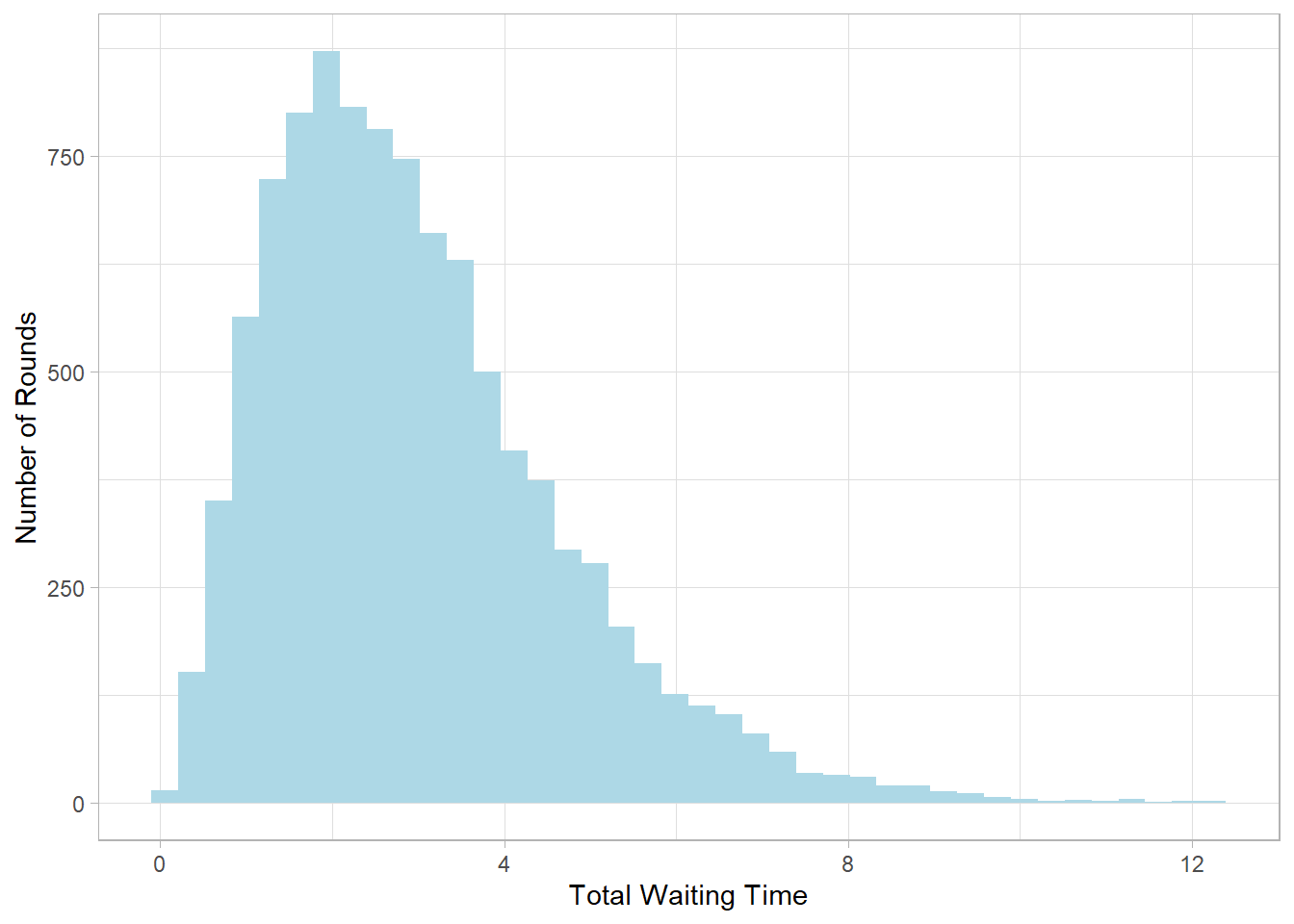
This histogram shows the distribution of total waiting times until the third customer arrives. Most values cluster around the center, with a tail extending to the right—typical of Gamma distributions when \(\alpha > 1\).
To calculate the exact probability density of waiting exactly 2
units of time (not probability of exactly 2, since this is a
continuous distribution), use the PDF via dgamma():
# Calculate the density at x = 2
dgamma(x = 2, shape = 3, rate = 1)
[1] 0.2706706
To find the cumulative probability of waiting up to
2 units of time, use pgamma():
# Cumulative probability of waiting ≤ 2 units
pgamma(q = 2, shape = 3, rate = 1)
[1] 0.3233236This gives the probability that the total waiting time for 3 customers will be 2 or less.
We can also find the 75th percentile—the waiting
time below which 75% of the values fall—using qgamma():
# 75th percentile of the Gamma distribution
qgamma(p = 0.75, shape = 3, rate = 1)
[1] 3.920402This helps interpret what a “typical” long wait might look like under this setup.
Now let’s turn to the Exponential distribution. As we discussed earlier, this is a special case of the Gamma distribution where \(\alpha=1\), meaning that we’re only waiting for one event to happen.
Suppose the average arrival rate is still 1 customer per unit time.
To simulate 10,000 waiting times for the
first customer, use rexp():
# Set seed
set.seed(123)

# Simulate 10,000 waiting times for 1 customer (rate = 1)
exp_sim <- rexp(n = 10000, rate = 1)

# Plot the simulated waiting times
tibble(x = exp_sim) %>%
  ggplot(aes(x = x)) +
  geom_histogram(fill = "skyblue", bins = 40) +
  labs(x = "Waiting Time for First Arrival",
       y = "Number of Rounds")
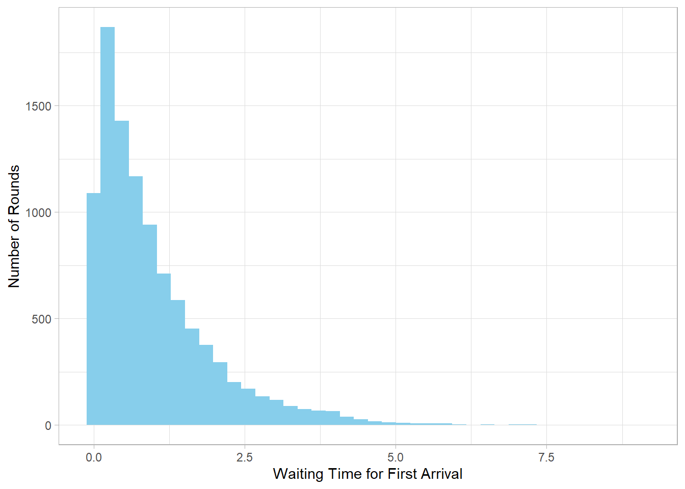
This histogram shows that short waiting times are more likely, but there’s still a long tail of possible longer waits—typical for Exponential distributions.
To compute the density (height of the PDF curve) at \(x = 2\):
# Density at x = 2
dexp(x = 2, rate = 1)
[1] 0.1353353To find the cumulative probability of waiting no more than 2 units:
# Cumulative probability of waiting ≤ 2 units
pexp(q = 2, rate = 1)
[1] 0.8646647And finally, to find the 75th percentile:
# 75th percentile of Exponential waiting times
qexp(p = 0.75, rate = 1)
[1] 1.386294This tells us that, in 75% of the cases, the waiting time will be below this value.
15.7 Recap
In this chapter, we explored two important continuous probability distributions: the Exponential and the Gamma. Both are closely related and are used to model waiting times and the timing of events.
The Exponential distribution focuses on the waiting time until the first event happens in a process where events occur continuously and independently at a constant rate. It’s widely used in fields like reliability testing, queuing theory, and survival analysis.
The Gamma distribution generalizes the Exponential by modeling the waiting time until the occurrence of multiple events. This makes it especially useful when we want to understand the total time for several independent events to happen, such as the time until the third customer arrives or the sum of multiple waiting periods.
Both distributions capture real-world processes involving time and randomness, with the Gamma building upon the simpler Exponential to handle more complex scenarios. Their mathematical properties and practical relevance make them essential tools for modeling durations and lifetimes in many applications.