In the previous chapter, we discussed the Binomial distribution, a
fundamental discrete distribution that models the number of
successes in a fixed number of independent trials. Building on that
foundation, this chapter introduces two closely related, discrete
distributions: the Poisson and the
Geometric distributions.
Both distributions can be understood as extensions of the ideas
behind the Binomial, but they describe different types of random
processes. To keep the concepts intuitive, we continue the coin-flip
story from the previous chapter, to illustrate how these
distributions arise naturally in simple, straightforward scenarios.
We also introduce their key statistical measures, such as expected
value and variance, and show how to perform simulations and
calculations using R. This hands-on approach will help you deepen
your understanding and apply these distributions in practical
situations.
14.2 When do we encounter
the Poisson distribution?
When the number of trials is large and the probability of success is
around 50%, the Binomial distribution becomes approximately Normal.
This makes intuitive sense as, when successes and failures are
equally likely, the outcomes tend to form a symmetric, bell-shaped
curve.
But what happens when the probability of success is very small?
Suppose we flip a (really) biased coin, where the chance of heads is
just 0.1%. In this case, getting a head can be seen as a
rare event. Even with many trials, successes will
be sparse and scattered.
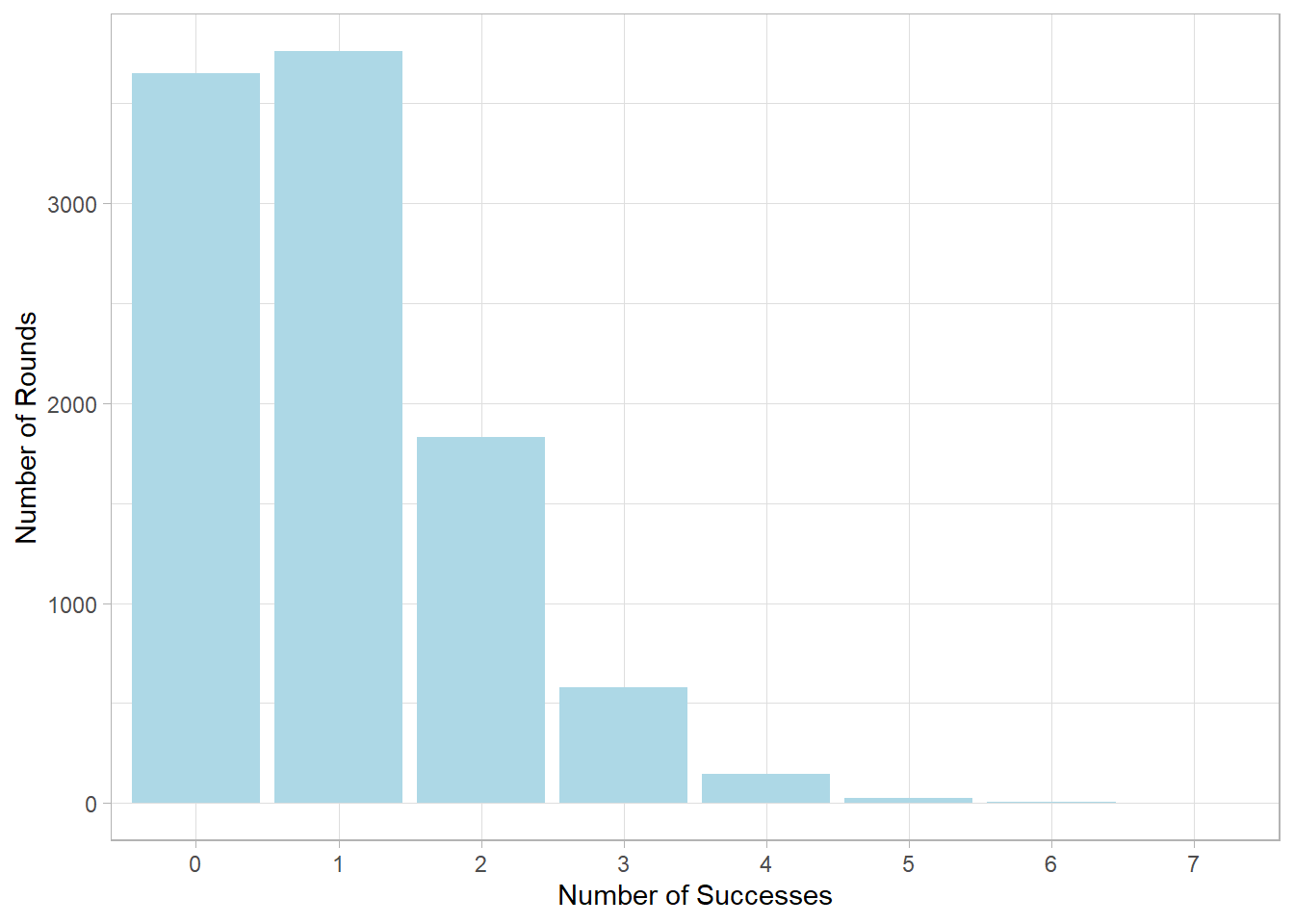
Let’s simulate this scenario. We’ll run 10,000 rounds, and in each
round we flip 1,000 coins where each flip has a 0.1% chance of
success. We then count how many successes occur in each round:
# Librarieslibrary(tidyverse)
── Attaching core tidyverse packages ──────────────────────── tidyverse 2.0.0 ──
✔ dplyr     1.1.4     ✔ readr     2.1.5
✔ forcats   1.0.1     ✔ stringr   1.5.2
✔ ggplot2   4.0.0     ✔ tibble    3.3.0
✔ lubridate 1.9.4     ✔ tidyr     1.3.1
✔ purrr     1.1.0
── Conflicts ────────────────────────────────────────── tidyverse_conflicts() ──
✖ dplyr::filter() masks stats::filter()
✖ dplyr::lag()    masks stats::lag()
ℹ Use the conflicted package (<http://conflicted.r-lib.org/>) to force all conflicts to become errors
# Setting the themetheme_set(theme_light())# Set seedset.seed(123)# Simulate 10000 rounds of 1000 coins with probability p = 0.001binomial_sim <-rbinom(10000, 1000, 0.001) # Plot the simulated counts as a bar charttibble(x =as.character(binomial_sim)) %>%ggplot(aes(x = x)) +geom_bar(fill ="lightblue") +labs(x ="Number of Successes",y ="Number of Rounds")
As you can see, the distribution of successes is far from Normal.
Most rounds result in zero or one success, with very few rounds with
more. Increasing the number of trials (e.g., more coin flip rounds)
won’t change this shape much, meaning that the asymmetry remains.
This is where the Poisson distribution comes in.
When the probability of success is very low and the number of trials
is very high, the Binomial distribution tends to converge to a
Poisson distribution. In simple terms, the Poisson distribution
models
how often a rare event happens, given many opportunities for it
to occur.
To make this more concrete, let’s look at a real-world example:
imagine a bookstore that receives, on average, 2 customer visits per
hour during late-night hours. Some hours may pass with no customers
at all, while others may see one, two, or occasionally even more.
Now, suppose we want to model the number of customer visits per
hour. Each visit is a relatively rare and random event, and we can
also assume that customers arrive independently of one another. This
is a perfect scenario for the Poisson distribution.
The Poisson distribution allows us to calculate the probability of
observing 0, 1, 2, or more events (in this case, visits) within a
fixed interval (one hour), given a known average rate (2 visits per
hour). For example, it can tell us how likely it is that no one
enters the store during a given hour, or that exactly three people
do.
14.3 What are the
parameters and shape of the Poisson distribution?
What makes the Poisson distribution particularly useful is that it
doesn’t require knowledge of how many “opportunities” for the event
there are (unlike the Binomial, which needs the number of trials).
Instead, it relies only on the rate at which the
events occur. The notation denoting a random variable
\(X\) following a Poisson
distribution is:
\[ X \sim Poisson(\lambda) \]
The parameter \(\lambda\) (lamda)
represents the average number of times an event happens
within a given interval. For example, if
\(\lambda = 3\), on average, we
expect 3 events to occur in that interval, though the actual number
in any one interval might be higher or lower. This average rate
\(\lambda\) is what makes the
Poisson distribution flexible and widely applicable, as it
summarizes how often events tend to happen without needing to know
the total number of possible trials.
But what exactly do we mean by a “fixed interval”? This interval can
be any well-defined segment of time, space, area, volume, or even
number of attempts, as long as it is clearly specified and
consistent across trials. For example, it could be one hour, during
which we count how many cars pass a checkpoint. It could also be one
square kilometer, where we count how many trees grow. Another
example is a day during which we count the number of customer
arrivals in a store. Or, as in our earlier example, it could be the
1,000 coin-flips in a single round.
Now, assuming we have a fixed and consistent interval, how do we
calculate the probability of observing a specific number of events,
say \(k\), given the average rate
\(\lambda\)? This is where we use
the probability mass function of the Poisson distribution:
\(k\) is the number of events
we want to find the probability for,
\(\lambda\) is the average rate
of events,
\(e\) is Euler’s number
(approximately 2.71828),
\(k!\) (\(k\)
factorial) is the product of all positive integers up to
\(k\).
To put this into context, let’s revisit our coin flip example from
earlier. We had 1,000 coins each with a 0.1% chance of landing
heads, so the expected number of heads (successes) per round was:
\[ \lambda = 1000 \times 0.001 = 1 \]
Using the PMF, we can calculate the probability of seeing exactly 0,
1, or 2 heads in one round:
So, even though each coin has a very small chance of landing heads,
the Poisson distribution lets us understand the probabilities of
different numbers of successes over many flips, based solely on the
average number of expected successes.
One of the interesting features of the Poisson distribution is that
its expected value and its variance are both equal to
\(\lambda\):
\[ E(X) = \lambda \]
\[ Var(X) = \lambda \]
This makes sense if we think about what
\(\lambda\) represents: it’s the
average number of times an event happens in a fixed
interval. Since it’s literally the average, it naturally becomes the
expected value. But, why is the variance also\(\lambda\)? Variance tells us how
spread out the values are around the mean. In a Poisson process,
events happen independently and randomly, but they follow a steady
(consistent) long-term rate. If events are truly rare and
independent, the variability in how many show up in each interval
should increase as the average number increases. So, if we expect
more events (\(\lambda\) is
higher), it’s also more likely that the number of events in each
interval will vary more. This is why the variance grows along with
the mean in a Poisson distribution—they’re tied together by the same
rate \(\lambda\).
14.4 When do we encounter
the Geometric distribution?
Let’s return to the coin-flipping example. Previously, we were
flipping coins a set number of times and counting how many of them
landed “heads”. That setup led us to the Binomial distribution,
which deals with counting successes across a fixed number of trials.
But now, let’s flip the question: instead of asking how many
successes we get after a fixed number of flips, let’s keep flipping
the coin until we get the first heads. In this
case, we’re no longer interested in how many successes (heads) we
get overall, but how long it takes to see the first one.
Imagine flipping a biased coin over and over, where the probability
of heads is 1%. On some tries, we might get heads immediately. Other
times, we might flip tails again and again before we finally get to
a head. Each flip is independent, and the chance of success stays
the same every single time.
This situation leads to the Geometric distribution.
It models how many failures we see before the first success. It’s a
natural fit when we’re dealing with repeated, independent attempts
at something—especially when that “something” doesn’t happen very
often. Below is the distribution of the Geometric random variable
when the probability of heads is 5%.
We can think of it as measuring the “waiting time” until a rare
event occurs (in essence, it is more like “waiting trials”).
It’s helpful to contrast the Geometric with the Poisson
distribution. While the Geometric distribution is about how many
failures occur before the first success, the Poisson
distribution is about how many successes occur
within a fixed interval of time or space. In short,
Geometric counts how long we wait for something to happen; Poisson
counts how often it happens within a given frame.
14.5 What are the
parameters and shape of the Geometric distribution?
We denote that a random variable
\(X\) follows a Geometric
distribution as:
\[ X \sim \text{Geometric}(p) \]
The parameter \(p\) represents the
probability of success on each individual trial.
For example, if \(p = 0.1\), each
trial has a 10% chance of success. As explained above then, the
Geometric distribution tells us how many
failures we would expect before we finally see one
success, and this is where the probability mass function (PMF) of
the Geometric distribution comes in:
\[ P(X = k) = (1 - p)^k p \]
Here:
\(k\) is the number of failures
before the first success (so
\(k\) = 0, 1, 2, …),
\(p\) is the probability of
success on a single trial,
\((1 - p)^k\) is the
probability of getting
\(k\) failures in a row before
that success.
As an example, suppose each trial has a 5% chance of success (\(p = 0.05\)). The probability of seeing success in the first try is:
\[ P(X = 0) = (1 - 0.05)^0 \times 0.05 = 0.05 \]
This is intuitive as the probability itself is 0.01. However, the
probability of seeing a success after a first failure is:
It is important to note that as the number of failures increases,
the probability of encountering a success
on that specific trial (i.e., after exactly
\(k\) failures) decreases
exponentially. But, importantly, the chance of success on any given
trial always remains \(p\).
Another interesting feature of the Geometric distribution is its
expected value and variance:
\[ E(X) = \frac{1 - p}{p} \]
\[ Var(X) = \frac{1 - p}{p^2} \]
These formulas also make intuitive sense. If
\(p\) is small (success is rare),
we should expect to wait longer for the first success, so the
expected number of failures increases. And because rare successes
can take wildly different numbers of attempts, the variance also
grows quickly when \(p\) is small.
This means that, on average, we expect 19 failures before success,
but the number could vary widely from one trial to the next.
14.6 Calculating and
Simulating in R
Base R provides built-in functions to work with both Poisson and
Geometric distributions. To explore how these functions work, let’s
revisit the examples from earlier in the chapter. We’ll start with
the Poisson distribution, then move on to the Geometric.
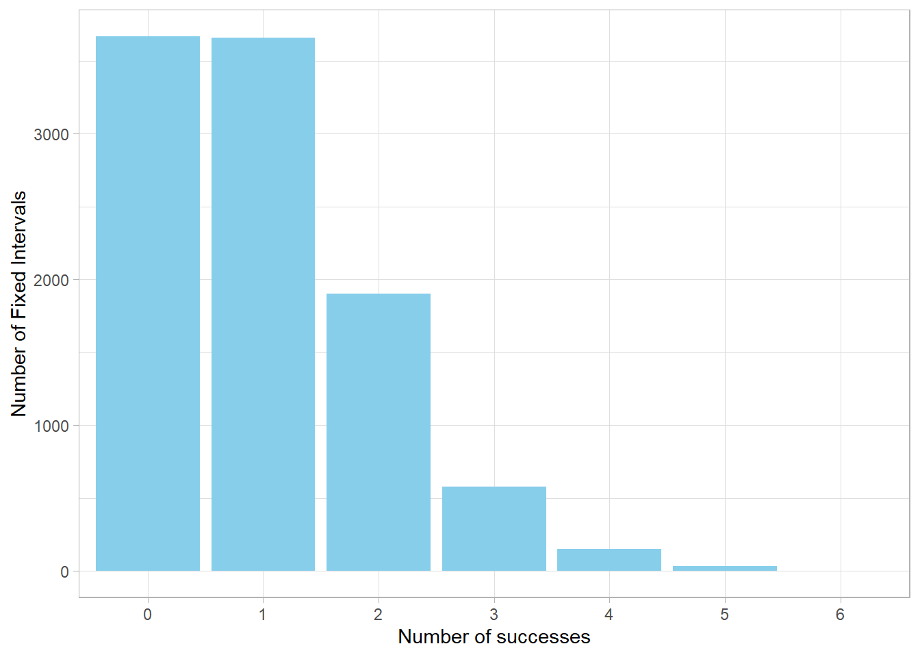
Let’s simulate the Poisson distribution example we discussed. Using
the rpois() function, we simulate 10,000 fixed
intervals (or rounds), each with an average event rate of
\(\lambda = 1\). Note that
\(\lambda = 1\) is the average
number of expected successes per round, obtained by multiplying the
small success probability (0.001) by the number of trials (1,000)
from our earlier example.
# Set seedset.seed(124)# Simulate 10,000 rounds with lambda = 1poisson_sim <-rpois(n =10000, lambda =1)# Plot the simulated counts as a bar charttibble(x =as.character(poisson_sim)) %>%ggplot(aes(x = x)) +geom_bar(fill ="skyblue") +labs(x ="Number of successes",y ="Number of Fixed Intervals")
The histogram you get from this simulation should look very similar
to the theoretical Poisson distribution we examined before.
To calculate the exact probability of observing exactly 1 success
when \(\lambda = 1\), use the
probability mass function with dpois():
# Calculate the probability of exactly 1 success when lambda = 1 using the PMFdpois(x =1, lambda =1)
[1] 0.3678794
This will return the same value we calculated earlier by hand.
To find the cumulative probability of getting up to 1 success with
the ppois() function:
# Calculate the cumulative probability of up to 1 successppois(q =1, lambda =1)
[1] 0.7357589
Recall from before that
\(P(X = 0) \approx 0.3679\) and
\(P(X = 1) \approx 0.3679\). Adding
these gives approximately 0.7358, which matches the output from
ppois().
Lastly, to find the value below which 75% of the data falls (the
75th percentile), use the quantile function qpois():
# Find the 75th percentile (quantile) of the Poisson distribution with lambda = 1qpois(p =0.75, lambda =1)
[1] 2
This number tells us that in about 75% of the intervals, the number
of successes will be less than or equal to this value, which makes
intuitive sense given the distribution’s shape and rate.
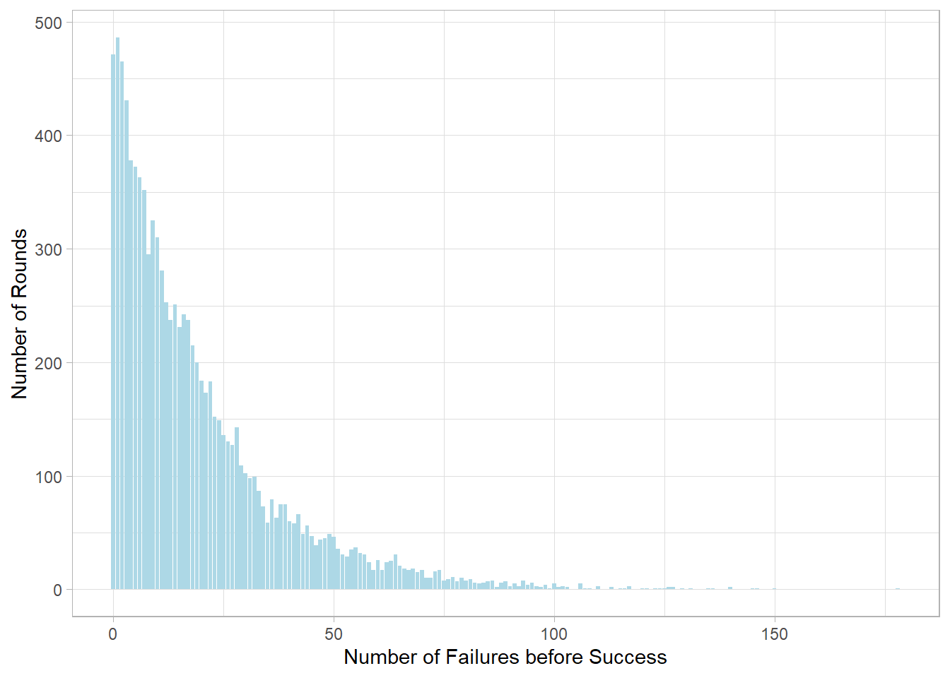
Next, let’s explore the Geometric distribution using R’s built-in
functions. To make a simulation, we use the
rgeom() function. For example, suppose the probability
of success (getting heads) on a coin flip is
\(p = 5\%\). We simulate 10,000
rounds of this process, each round representing a sequence of flips
until the first head appears.
# Set seedset.seed(123)# Simulate 10,000 trials with success probability 5%geometric_sim <-rgeom(10000, 0.05) # Plot the distribution of the number of failures before the first successtibble(x = geometric_sim) %>%ggplot(aes(x = x)) +geom_bar(fill ="lightblue") +labs(x ="Number of Failures before Success",y ="Number of Rounds")
This histogram shows how often we observe a certain number of
failures before the first success when the success probability is
very low. Notice how the bars decline as the number of failures
increases, illustrating that longer waiting times for success are
less likely.
We can calculate the probability of having exactly
\(k\) failures before the first
success using the probability mass function with
dgeom():
# Calculate probability of 5 failures before success (p = 0.05)dgeom(x =5, prob =0.05)
[1] 0.03868905
This gives the probability of waiting exactly 5 failures before the
first success occurs.
Similarly, to find the cumulative probability of having up to
\(k\) failures before the first
success, we use the pgeom() function:
# Calculate cumulative probability of up to 5 failures before successpgeom(q =5, prob =0.05)
[1] 0.2649081
We can confirm this by filtering our simulated data and calculating
the proportion of rounds with 5 or fewer failures:
# Proportion of simulated rounds with 5 or fewer failuressum(geometric_sim <=5) /length(geometric_sim)
[1] 0.2603
Finally, to find the quantile (the number of failures below which a
certain percentage of outcomes fall), use qgeom(). For
example, the 75th percentile tells us the number of failures we
expect to see in 75% of the rounds:
# Find the 75th percentile of failures before successqgeom(p =0.75, prob =0.05)
[1] 27
14.7 Recap
In this chapter, we explored two important discrete probability
distributions: the Poisson and the Geometric. Both extend the ideas
behind the Binomial distribution but focus on different aspects of
random events.
The Poisson distribution helps us understand how often rare events
happen over a fixed interval of time or space, without needing to
know the exact number of trials. It’s widely used in real-life
situations like counting customer arrivals, phone calls, or defects
in manufacturing.
The Geometric distribution, on the other hand, models the waiting
time (trials to be exact) until the first success, or equivalently,
the number of failures before that success occurs. This makes it
valuable when we want to measure “how long” or “how many tries” it
takes to get something to happen for the first time.
Both distributions share an intuitive connection to real-world
processes involving rare events and independent trials. Their
mathematical simplicity, combined with their practical usefulness,
makes them fundamental tools for understanding and modeling
randomness in many fields.